Overview
For the first lab, we’ll be using a commonly-used dataset in many data science tutorials!
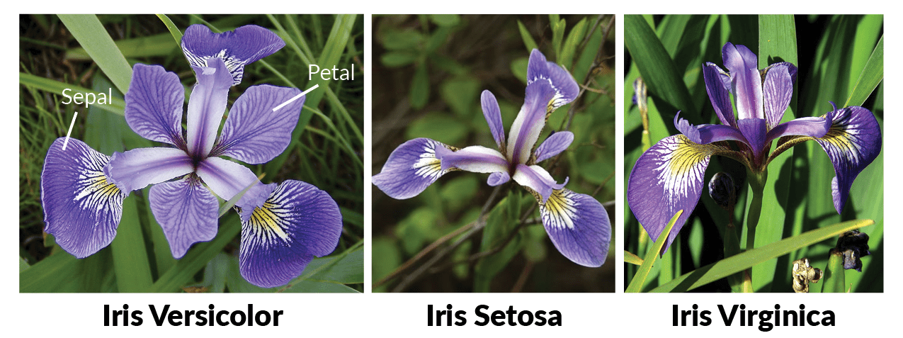
The IRIS dataset is a well known dataset introduced by Ronald Fisher in his 1936 paper. This dataset contains three plant species (setosa, virginica, versicolor) and four features measured (Sepal.Length, Sepal.Width, Petal.Length, Petal.Width). For each sample, all measurements of each feature are given in centimeters.
R summary of the data
Using the str() function, we’ll let R list out the variables and its individual data types in the IRIS dataset.
'data.frame':   150 obs. of  5 variables:
 $ Sepal.Length: num  5.1 4.9 4.7 4.6 5 5.4 4.6 5 4.4 4.9 ...
 $ Sepal.Width : num  3.5 3 3.2 3.1 3.6 3.9 3.4 3.4 2.9 3.1 ...
 $ Petal.Length: num  1.4 1.4 1.3 1.5 1.4 1.7 1.4 1.5 1.4 1.5 ...
 $ Petal.Width : num  0.2 0.2 0.2 0.2 0.2 0.4 0.3 0.2 0.2 0.1 ...
 $ Species     : Factor w/ 3 levels "setosa","versicolor",..: 1 1 1 1 1 1 1 1 1 1 ...
Meanwhile, calling head() will give us direct view access to the first few rows in the dataset, allowing us to see the clear formatting:
| 5.1 |
3.5 |
1.4 |
0.2 |
setosa |
| 4.9 |
3.0 |
1.4 |
0.2 |
setosa |
| 4.7 |
3.2 |
1.3 |
0.2 |
setosa |
| 4.6 |
3.1 |
1.5 |
0.2 |
setosa |
| 5.0 |
3.6 |
1.4 |
0.2 |
setosa |
| 5.4 |
3.9 |
1.7 |
0.4 |
setosa |
We see that the IRIS dataset is mostly made of numerical variables, which represent the physical features of an iris flower (in centimenters). Additionally, there is one categorical variable, species, can only take values within a set (in this case, it would be the individual iris species types).
Figure 1: Iris Flowers (Willems, 2018)