While linear regression does well at predicting the value of a numerical dependent variable, it doesn’t cover the scenario where the dependent outcome could be categorical, such as a binary outcome (for example, ‘yes’ or ‘no’).
In these cases, we’d use logistic regression instead, where we calculate the probability of the dependent outcome occurring.
An example of a logistic regression curve (Kanade, V. 2022. Spiceworks.)
Predicting Direction using Logistic Regression
In this section, we’ll be using the Smarket dataset to fit a logistic regression model, glm.fits. Our goal is to predict Direction using the variables Lag1 through Lag5 and Volume.
To do this, we’ll utilize the glm() function, which can fit many types of generalized linear models, including logistic regression.
glm() functions similarly to lm(), with the difference being that we’d need to specify family = binomial in order to let R know we are running a logistic regression and not a generalized linear model.
Call:
glm(formula = Direction ~ Lag1 + Lag2 + Lag3 + Lag4 + Lag5 +
    Volume, family = binomial, data = Smarket)

Coefficients:
             Estimate Std. Error z value Pr(>|z|)
(Intercept) -0.126000   0.240736  -0.523    0.601
Lag1        -0.073074   0.050167  -1.457    0.145
Lag2        -0.042301   0.050086  -0.845    0.398
Lag3         0.011085   0.049939   0.222    0.824
Lag4         0.009359   0.049974   0.187    0.851
Lag5         0.010313   0.049511   0.208    0.835
Volume       0.135441   0.158360   0.855    0.392

(Dispersion parameter for binomial family taken to be 1)

    Null deviance: 1731.2  on 1249  degrees of freedom
Residual deviance: 1727.6  on 1243  degrees of freedom
AIC: 1741.6

Number of Fisher Scoring iterations: 3
The smallest p-value in glm.fits is associated with Lag1. The negative coefficient for this predictor suggests that if the market had a positive return yesterday, then it’s less likely to go up today. However at a value of 0.15, the p-value is still considered relatively large (especially at a 95% confidence level), and so there is no clear evidence of a real association between Lag1 and Direction.
We’ll use the coef() function in order to access just the coefficients for this fitted model. We can also use the summary() function to access particular aspects of the fitted model, such as the p-values for the coefficients.
rbind(coef(glm.fits))
(Intercept)
Lag1
Lag2
Lag3
Lag4
Lag5
Volume
-0.1260003
-0.0730737
-0.0423013
0.0110851
0.0093589
0.0103131
0.1354407
round(summary(glm.fits)$coef, 4)
Estimate
Std. Error
z value
Pr(>|z|)
(Intercept)
-0.1260
0.2407
-0.5234
0.6007
Lag1
-0.0731
0.0502
-1.4566
0.1452
Lag2
-0.0423
0.0501
-0.8446
0.3983
Lag3
0.0111
0.0499
0.2220
0.8243
Lag4
0.0094
0.0500
0.1873
0.8514
Lag5
0.0103
0.0495
0.2083
0.8350
Volume
0.1354
0.1584
0.8553
0.3924
The predict() function will predict the probability that the market will go up, given values of the predictors. When we use type = "response" as a parameter with predict(), it tells R to output probabilities of the form P(Y = 1/X), as opposed to other information such as the logit. If no dataset is supplied to the predict() function, then the probabilities are computed for the training data that was used to fit the logistic regression model.
Here, we’ve printed the first ten probabilities. We know that these values correspond to the probability of the market going up, rather than down, because the contrasts() function indicates that R has created a dummy variable with the value 1 for up.
The diagonal elements of the confusion matrix (Down*Down, Up*Up) indicate the number of correct predictions, while the off-diagonals represent incorrect predictions. This means our model correctly predicted that the market would go up on 507 days, and that it would go down on 145 days, for a total of (507 + 145) 652 correct predictions.
The mean() function can be used to compute the fraction of days for which the predictions were correct:
(145+507)/length(Smarket$Direction)
[1] 0.5216
In this case, our model correctly predicted the movement of the market 52.2% of the time.
Another way to find the overall prediction accuracy level
mean(glm.pred==Smarket$Direction)
So far, in the above model, we’ve trained it using the whole sample for an accuracy level of 52.2%, however, this implies that we have a 47.8% training error rate which is not good. How can we improve that?
Data splitting and subsetting
To better assess the accracy of logistic regression model data, we’ll utilize the methods shown in KNN training where we split the data in Smarket into train and test subsets. This will give us a more realistic error rate, as these types of models are often used to predict future events, not data that it had already been trained on.
Years 2001-2004 will be used to train the logistic regression model, while 2005 will be the test data.
Now that we’ve trained our model from data in 2001-2004, we’ll test it using the 2005 data, which is a completely separate dataset. The predictions for 2005 will be computed and compared to the actual movements of the market in that time period.
The results happen to be rather disappointing, with the test error rate equating to 52% (accuracy rate of 48%), which is worse than random guessing. This result isn’t all that surprising, though, given that you’d generally not expect to be able to use previous days’ returns to predict future market performance.
However, let’s consider using only Lag1 and Lag2 in the model, which means we’ll only consider the returns of the last two days in our data.
glm.fits3 =glm(Direction~Lag1 + Lag2,data=train,family=binomial)glm.probs3 =predict(glm.fits3, test,type="response")glm.pred3 =ifelse(glm.probs3>0.5, "Up","Down")# Confusion matrixtable(glm.pred3,test$Direction)# Accuracy rateround( mean(glm.pred3 == test$Direction), 2) # error rate# Success rate for days with 'Up'round( 106/(106+76) ,2 )
Confusion Matrix
Down
Up
Down
35
35
Up
76
106
0.56
0.58
The new results seem to be somewhat better: 56% of the daily directions have been correctly predicted, and on days where they predict an increase in the market, the accuracy rate is 58%.
Getting the ROC curve
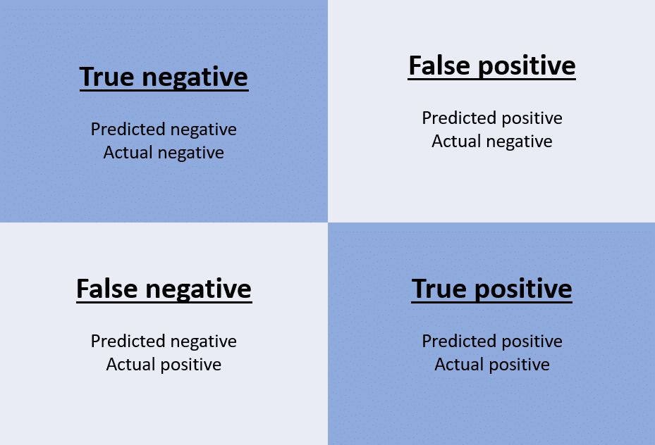
A ROC curve stands for a “receiver operating characteristic curve”, and graphs the performance of a classification model’s false positive and false negative rate.
To get the ROC graph, we’ll have to first install the package pROC.
library(pROC) # install.packages("pROC")library(ISLR2)# Up = 2 (the case level)# Down = 1 (the control level)test$Direction[1:5]as.numeric(test$Direction[1:5])
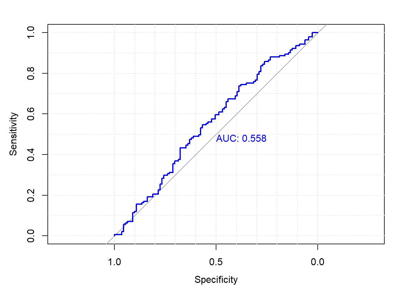
The AUC value (area under the curve) is sometimes used to summarize the overall performance. A higher AUC value is good.
What we can surmise from the code and output above:
Sensitivity: the probability of a true positive
Specificity: the probability of a true negative
plot = TRUE will give us the ROC plot
print.auc = TRUE will print out the area under the curve
An AUC of 0.558 tells us that our model is slightly better at predicting than random guessing would be.
Making Specific Predictions with a Logistic Regression Model
Let’s say we want to predict the direction on a day where Lag1 = (1.2, 1.5), and Lag2 = (1.1, -0.8). We are able to do that by creating a dataframe with the specific Lag1 and Lag2 values we want.