Discriminant Analysis

Like logistic regression, linear discriminant analysis (LDA) aims to classify observations where the dependent variable is categorical. The main difference between the two types of models is that logistic regression is often used to find the most important predictors, or seeing how the different variables play in prediction, while discriminant analysis has emphasis on the categorical prediction itself.

Additionally, discriminant analysis makes more assumptions about the underlying data compared to logistic regression. For example, LDA assumes that the predictor variables are normally distributed and have equal variance-covariance matrices across groups. Logistic regression doesn’t make these assumptions about the predictor variables, and is therefore considered more flexible with fewer assumptions about the underlying data distribution.

Linear and quadratic discriminant analysis example (2021. Machine Learning Explained.)

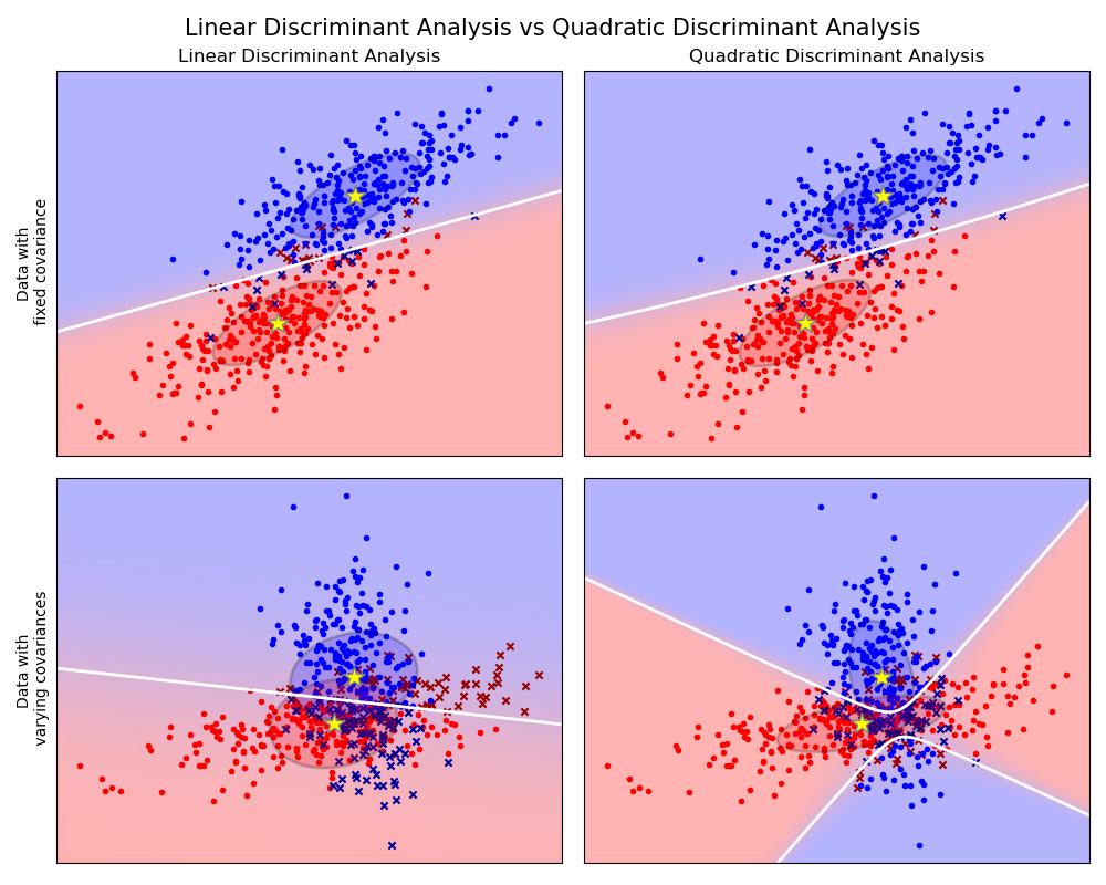
Discriminant analysis works by constructing a hyperplane between two groups that acts as a boundary between classification groups.

A hyperplane is a boundary that divides an input space into two or more regions. It is always one dimension less than the input space (i.e., a line in a 2D space, separating it, or a plane in a 3D space.)

Hyperplane examples (2024. GeeksForGeeks.)

Linear Discriminant Analysis

To perform Linear discriminant analysis (LDA) in R, we need the lda() function, which is a part of the MASS library. Note that the syntax for the lda() function is nearly identical to lm() and glm() except for the absence of the family option.

We’ll be using the Smarket dataset dataset to fit the model, and this time, we’ll only be using the observations before 2005. Our code and models continue from our logistic regression examples, and some variables, such as the training and test set, are defined there.

library(MASS)
lda.fit = lda(Direction~Lag1 + Lag2, data = train)
lda.fit

Call:
lda(Direction ~ Lag1 + Lag2, data = train)

Prior probabilities of groups:
    Down       Up 
0.491984 0.508016 

Group means:
            Lag1        Lag2
Down  0.04279022  0.03389409
Up   -0.03954635 -0.03132544

Coefficients of linear discriminants:
            LD1
Lag1 -0.6420190
Lag2 -0.5135293

The prior probability of groups are \^{\pi_1} = 0.492 and \^{\pi_2} = 0.508. In other words, 49.2% of the training observations correspond to days during which the market went down.

The group means are the average of each predictor within the classes, and are used by LDA as estimates of \mu_k. These suggest that there is a tendency for the previous 2 days’ returns to be negative on days when the market increases, and a tendency for the previous days’ returns to be positive on days when the market declines.

The coefficients of linear discriminants provide the linear combination of Lag1 and Lag2, that are used to form the LDA decision rule, a linear combination of the predictors that maximally separates the groups (Down and Up) in the LDA model. In other words, the decision boundary is:

-0.642 * Lag1 - 0.541*Lag2

Observations above this boundary line are more likely to be classified as Up, and those below, are more likely to be classified as “Down”.

plot(lda.fit)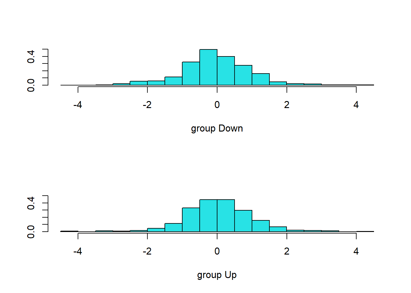

The plot() function produces plots of the linear discriminants, obtained by computing the boundary equation for each of the training observations.

lda.pred = predict(lda.fit, test)
names(lda.pred)

[1] "class"     "posterior" "x"        

# Try calling on lda.pred and see the output for yourself!

The predict() function returns a list with three elements:

• class: LDA’s predictions about the market movement (Up, Down).
• posterior: a matrix whose k^{th} column contains the posterior probability that the corresponding observation belongs in the k^{th} class.
• x: the linear discriminants.

lda.class = lda.pred$class
table(lda.class, test$Direction)

# Overall prediction accuracy level
mean(lda.class== test$Direction)

	Down	Up
Down	35	35
Up	76	106

[1] 0.5595238

When taking the accuracy scores from the logistic regression model example, we see that the LDA and logistic regression prediction scores are similar, with approximately 56% accuracy for both.

Posterior Probabilities in LDA

The code below shows the predictions for the first five rows of the test observations. In all of them, the probability for Up is greater than 50%, which is why all of the predictions are also for Up.

# Displays the first 5 rows of posterior probabilities
lda.pred$post[1:5,]

	Down	Up
999	0.4901792	0.5098208
1000	0.4792185	0.5207815
1001	0.4668185	0.5331815
1002	0.4740011	0.5259989
1003	0.4927877	0.5072123

lda.pred$class[1:5]

[1] Up Up Up Up Up
Levels: Down Up

The calculations below show the link between LDA classifications and posterior probabilities, by cross-referencing the similarity between row counts and classifications.

• The number of cases where the posterior probability >= 0.5 will be the same as the number of predictions for Up the LDA made.
• The number of cases where the posterior probability < 0.5 will also be the same as the number of predictions for Down the LDA made.

length(test$Direction)

[1] 252

# The number of cases where the posterior prob >= 0.5 
# = number(Down->Up, Up->Up),
# = the sum of first row of confusion matrix
sum(lda.pred$post[,1]>=0.5) 

[1] 70

# The number of cases that posterior prob <0.5 
# = number (Down->Down, Up-> Down)
# = the sum of 2nd row of confusion matrix
sum (lda.pred$posterior[, 1] < 0.5)

[1] 182

182 + 70 = 252

lda_rox = roc(as.numeric(test$Direction)~lda.pred$post[,2], 
              plot = TRUE,col="blue",
              grid = TRUE,
              print.auc = TRUE)

Setting levels: control = 1, case = 2

Setting direction: controls < cases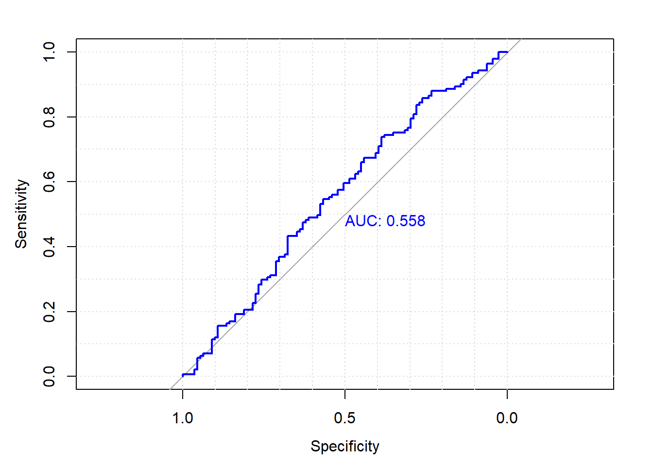

Quadratic Discriminant Analysis

When a linear boundary equation may not fit the data well, discriminant analysis of higher powers may show an improvement over LDA.

We will now fit a quadratic discriminany analysis (QDA) model to the Smarket dataset. QDA is implemented in R with the qda() function, which is also part of the MASS library. Note that the qda() syntax is the same as lda().

qda.fit = qda (Direction ~ Lag1 + Lag2 , data = train)
qda.fit

Call:
qda(Direction ~ Lag1 + Lag2, data = train)

Prior probabilities of groups:
    Down       Up 
0.491984 0.508016 

Group means:
            Lag1        Lag2
Down  0.04279022  0.03389409
Up   -0.03954635 -0.03132544

qda.pred = predict(qda.fit,test)
names(qda.pred)

[1] "class"     "posterior"

qda.class = qda.pred$class
table(qda.class,test$Direction)

         
qda.class Down  Up
     Down   30  20
     Up     81 121

mean(qda.class==test$Direction) # overall accuracy

[1] 0.5992063

mean(qda.class!=test$Direction) # error rate

[1] 0.4007937

qda.pred$post[1:10,]

          Down        Up
999  0.4873243 0.5126757
1000 0.4759011 0.5240989
1001 0.4636911 0.5363089
1002 0.4739253 0.5260747
1003 0.4903426 0.5096574
1004 0.4913561 0.5086439
1005 0.4922951 0.5077049
1006 0.4847447 0.5152553
1007 0.4889595 0.5110405
1008 0.4818971 0.5181029

qda_rov = roc(as.numeric(test$Direction)~qda.pred$post[,2],
              plot = TRUE,col="blue",
              grid = TRUE,
              print.auc = TRUE)

Setting levels: control = 1, case = 2

Setting direction: controls < cases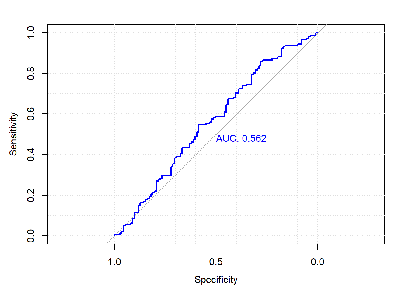

Key differences between LDA and QDA

1. Covariance matrices: LDA assumes equal covariance matrices across classes, while QDA allows different covariance matrices for each class.

2. Decision boundaries: LDA produces linear decision boundaries, whereas QDA produces quadratic decision boundaries.

3. Model complexity: LDA is less complex and has fewer parameters compared to QDA, making it less flexible but potentially more stable with small sample sizes.

4. Flexibility: QDA is more flexible and can model complex relationships between the predictor variables and the class labels but may require more data to estimate the additional parameters accurately.

Naive Bayes

The Naive Bayes models compared to discriminant analysis have many similarities; namely, they both use probabilistic approaches (posterior probability), however they differ in how they calculate the probabilities for classification.

Namely, Naive Bayes assumes all observation features are independent in each class and functions well when the number of features is large. Despite the strong assumptions, Naive Bayes often produces good classification results when the data fits the requirements to make it work.

We’ll fit a Naive Bayes model to the Smarket data. Naive Bayes is implemented in R using the naiveBayes() function, which is part of the e1071 library. The syntax is identical to that of lda() and qda().

library(e1071)
nb.fit = naiveBayes (Direction ~ Lag1 + Lag2 , data = train)
nb.fit

Naive Bayes Classifier for Discrete Predictors

Call:
naiveBayes.default(x = X, y = Y, laplace = laplace)

A-priori probabilities:
Y
    Down       Up 
0.491984 0.508016 

Conditional probabilities:
      Lag1
Y             [,1]     [,2]
  Down  0.04279022 1.227446
  Up   -0.03954635 1.231668

      Lag2
Y             [,1]     [,2]
  Down  0.03389409 1.239191
  Up   -0.03132544 1.220765

The output contains the estimated mean and standard deviation for each variable in each class. For example, the mean for Lag1 is 0.0428 when the direction is Down, and the standard deviation is 1.23.

We can easily verify this:

# mean/sd of Lag1 that meets condition: Direction=="Down"
mean(train$Lag1[train$Direction =="Down"]) 

[1] 0.04279022

sd(train$Lag1[train$Direction =="Down"])

[1] 1.227446

The predict() function is straightforward, providing us with a confusion matrix on the classifications of the Naive Bayes model.

nb.class = predict(nb.fit,test)
table(nb.class,test$Direction)

mean(nb.class==test$Direction) # Accuracy
mean(nb.class!=test$Direction) # Error rate

Confusion Matrix

	Down	Up
Down	28	20
Up	83	121

[1] 0.5912698

Naive Bayes performs well on this data compared to LDA and Logistic Regression, though slightly worse than QDA, when comparing the accuracy rates.

The predict() function can also generate estimates of the probability that each observation belongs to a particular class.

nb.preds = predict(nb.fit, test, type = "raw")
nb.preds[1:5,]

Down	Up
0.4873164	0.5126836
0.4762492	0.5237508
0.4653377	0.5346623
0.4748652	0.5251348
0.4901890	0.5098110

nb_roc = roc(as.numeric(test$Direction)~nb.preds[,2],
             plot = TRUE,col="blue",
             grid = TRUE,
             print.auc = TRUE)

Setting levels: control = 1, case = 2

Setting direction: controls < cases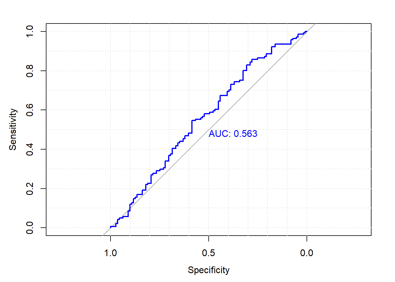

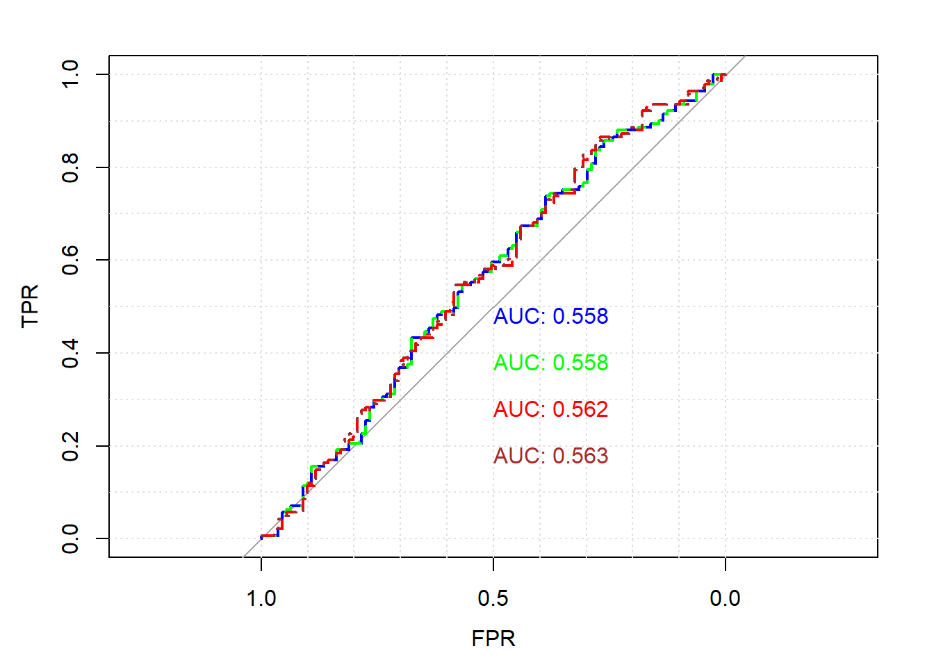
Plotting Multiple ROC Curves on the Same Graph

When passing a ROC objecting into plot(), it comes with a parameter called add, which when marked “T” (stands for true), tells R to keep the previous plot and put the current ROC curve on it as well.

• print.auc.y is a parameter that allows us to specify where on the y-axis the AUC value lies, in order to prevent overlapping.
• col functions as usual, allowing us to choose the color of the ROC curve when given a color.

You may or may not need to call plot.new() to clear all plots before starting.

plot.new()

plot(roc(as.numeric(test$Direction), glm.probs3), 
         xlab="FPR", ylab="TPR",print.auc = TRUE, grid=T, col = "blue")

plot(roc(as.numeric(test$Direction)~lda.pred$post[,2]),lty=2,print.auc=T, 
        col = "green", print.auc.y = .4, add = T)

plot(roc(as.numeric(test$Direction)~qda.pred$post[,2]),lty=2,print.auc=T, 
        col = "red", print.auc.y = .3, add = T)

plot(roc(as.numeric(test$Direction)~nb.preds[,2]),lty=3,print.auc=T, 
        col = "brown", print.auc.y = .2, add = T)

Linear and quadratic discriminant analysis example (2021. Machine Learning Explained.) Hyperplane examples (2024. GeeksForGeeks.)