The Smarket Dataset

For this lab, we’ll begin by examining some numerical and graphical summaries of the Smarket data, which is accessible via the ISLR2 library. The dataset consists of percentage returns for the S&P 500 stock index over 1,250 days, from the beginning of 2001 to the end of 2005.

For each date,

Lag1 through Lag5 record the percentage returns for each of the five previous days.
Volume represents the number of shares traded on the previous day, in billions.
Today represents the percentage return on the date in question.
Direction represents whether the market was up or down on this date.

Our goal using this dataset will be to predict Direction (a qualitative response) using the other features. To accomplish this, we’ll utilize the logistic regression model and linear discriminant analysis (LDA) or quadratic discriminant analysis (QDA).

library(ISLR2)
str(Smarket)

'data.frame':   1250 obs. of  9 variables:
 $ Year     : num  2001 2001 2001 2001 2001 ...
 $ Lag1     : num  0.381 0.959 1.032 -0.623 0.614 ...
 $ Lag2     : num  -0.192 0.381 0.959 1.032 -0.623 ...
 $ Lag3     : num  -2.624 -0.192 0.381 0.959 1.032 ...
 $ Lag4     : num  -1.055 -2.624 -0.192 0.381 0.959 ...
 $ Lag5     : num  5.01 -1.055 -2.624 -0.192 0.381 ...
 $ Volume   : num  1.19 1.3 1.41 1.28 1.21 ...
 $ Today    : num  0.959 1.032 -0.623 0.614 0.213 ...
 $ Direction: Factor w/ 2 levels "Down","Up": 2 2 1 2 2 2 1 2 2 2 ...

head(Smarket, n=5)

Year	Lag1	Lag2	Lag3	Lag4	Lag5	Volume	Today	Direction
2001	0.381	-0.192	-2.624	-1.055	5.010	1.1913	0.959	Up
2001	0.959	0.381	-0.192	-2.624	-1.055	1.2965	1.032	Up
2001	1.032	0.959	0.381	-0.192	-2.624	1.4112	-0.623	Down
2001	-0.623	1.032	0.959	0.381	-0.192	1.2760	0.614	Up
2001	0.614	-0.623	1.032	0.959	0.381	1.2057	0.213	Up

summary(Smarket)

Summary Statistics
Variable	N	Mean	Std. Dev.	Min	Pctl. 25	Pctl. 75	Max
Year	1250	2003	1.4	2001	2002	2004	2005
Lag1	1250	0.0038	1.1	-4.9	-0.64	0.6	5.7
Lag2	1250	0.0039	1.1	-4.9	-0.64	0.6	5.7
Lag3	1250	0.0017	1.1	-4.9	-0.64	0.6	5.7
Lag4	1250	0.0016	1.1	-4.9	-0.64	0.6	5.7
Lag5	1250	0.0056	1.1	-4.9	-0.64	0.6	5.7
Volume	1250	1.5	0.36	0.36	1.3	1.6	3.2
Today	1250	0.0031	1.1	-4.9	-0.64	0.6	5.7
Direction	1250
... Down	602	48%
... Up	648	52%

Getting the Down and Up Data Distribution

table(Smarket$Direction)/nrow(Smarket)


  Down     Up 
0.4816 0.5184

The cor() function produces a matrix of the numerical predictors in a dataset. Since Direction is not a numerical variable, we’ll need to drop it to get the correlation matrix.

cnames = colnames(Smarket)
round(cor(Smarket[, cnames != "Direction"]), 4)

	Year	Lag1	Lag2	Lag3	Lag4	Lag5	Volume	Today
Year	1.0000	0.0297	0.0306	0.0332	0.0357	0.0298	0.5390	0.0301
Lag1	0.0297	1.0000	-0.0263	-0.0108	-0.0030	-0.0057	0.0409	-0.0262
Lag2	0.0306	-0.0263	1.0000	-0.0259	-0.0109	-0.0036	-0.0434	-0.0103
Lag3	0.0332	-0.0108	-0.0259	1.0000	-0.0241	-0.0188	-0.0418	-0.0024
Lag4	0.0357	-0.0030	-0.0109	-0.0241	1.0000	-0.0271	-0.0484	-0.0069
Lag5	0.0298	-0.0057	-0.0036	-0.0188	-0.0271	1.0000	-0.0220	-0.0349
Volume	0.5390	0.0409	-0.0434	-0.0418	-0.0484	-0.0220	1.0000	0.0146
Today	0.0301	-0.0262	-0.0103	-0.0024	-0.0069	-0.0349	0.0146	1.0000

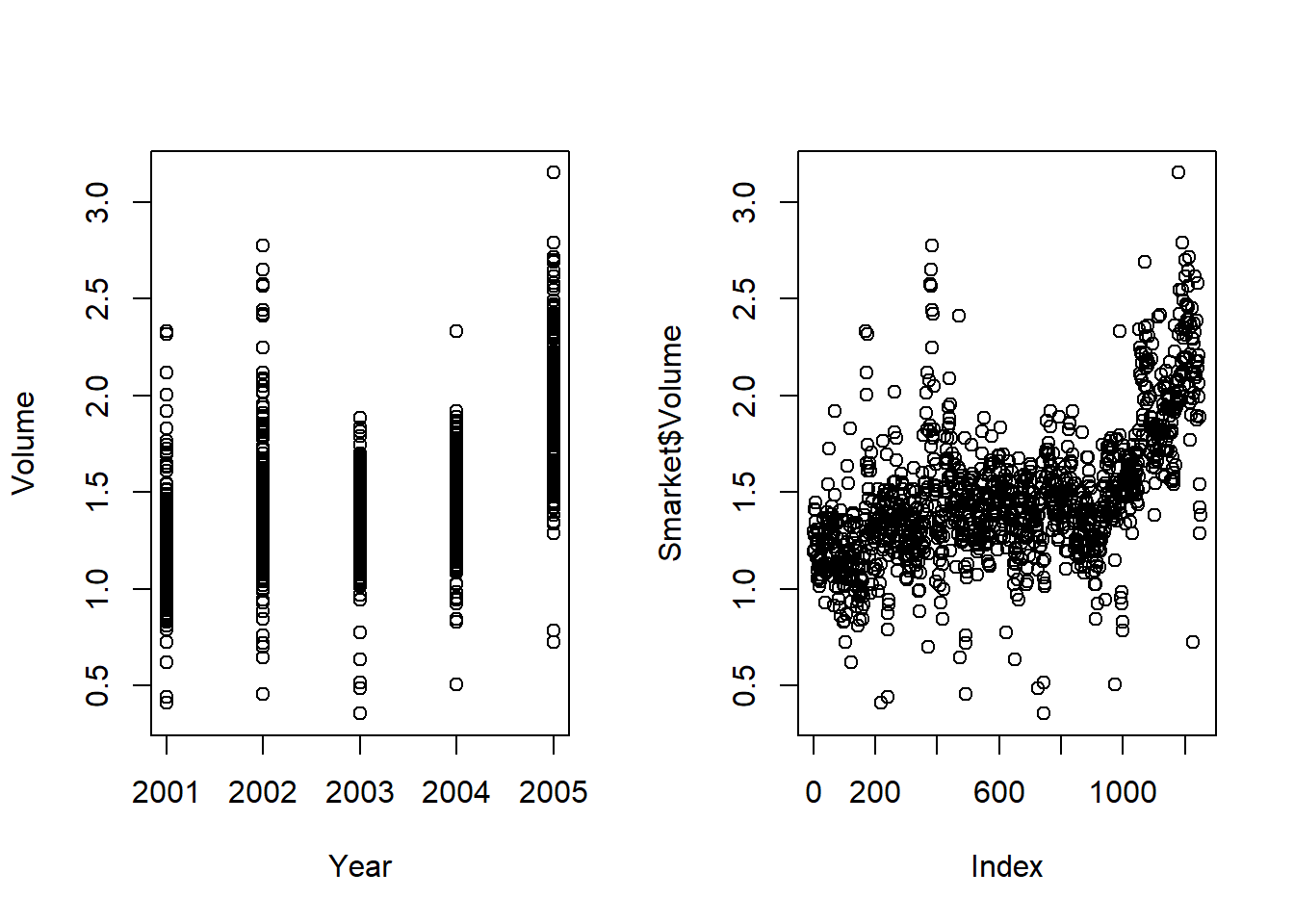
As one would expect, the correlations between the lag variables and today’s return are close to zero. In other words, there appears to be little correlation between today’s return and previous days’ returns. The only substantial correlation is between Year and Volume. By plotting the data, which is ordered chronologically, we see that Volume is increasing over time. In other words, the average number of shares traded daily increased from 2001 to 2005.

par(mfrow=c(1,2))
plot(Volume~Year, data=Smarket)
plot(Smarket$Volume)