Model Selection

When creating a multiple linear regression model, how do we know which combination of independent variables will yield us the best model?

There are two main ways of assessing independent variables in model selection:

1. Relevance to the research context: when we are designing experiments, we should have a logical idea of which variables we are more interested in looking at. However, we might not always have the research context, which brings us to option 2.
2. Statistical Significance: we can assess the model’s performance using metrics such as the AIC, BIC, R-squared, and adjusted R-squared values.

To summarize what each individual model-assessing metric means, the explanations will be listed below.

• R-squared: The coefficient of determination. This number represents the proportion of the variation in the dependent variable that’s predictable from the independent variable.
• Adjusted R-squared: The modified version of R-squared that accounts for the number of predictors in the model. While R-squared is suitable for models with one predictor, the adjusted R-squared value is suitable for models with multiple predictors.
• AIC: Stands for the Akaike Information Criterion. This is an estimator of prediction error, giving a relative quality score of statistical models for a given set of data.
• BIC: Stands for Bayesian Information Criterion. The BIC scores a finite set of models, where lower scores are preferred, and is based on the likelihood function.
• Cp: Known as Mallow’s C_p. A smaller value indicates that the model has small variance and is relatively precise.

Packages

There are two packages we will make use of, namely:

• MASS, which contains a large amount of datasets and functions.
• ISLR2, containing widely used datasets which we operate on.

library(MASS)
library(ISLR2)

Continuing from simple linear regression we will once again use the Boston Housing dataset in these examples.

Finding the Correlation Matrix

First, we examine the correlation between all numerical variables in the Boston dataset.

Before we apply the cor() function, we need to list all the numerical variables and assign it to an object, denoted Cols.

Cols = c('crim', 'zn', 'indus', 'nox', 'rm', 'age', 'dis', 'rad', 'tax', 'ptratio','lstat', 'medv')

head(Boston[Cols])

crim	zn	indus	nox	rm	age	dis	rad	tax	ptratio	lstat	medv
0.00632	18	2.31	0.538	6.575	65.2	4.0900	1	296	15.3	4.98	24.0
0.02731	0	7.07	0.469	6.421	78.9	4.9671	2	242	17.8	9.14	21.6
0.02729	0	7.07	0.469	7.185	61.1	4.9671	2	242	17.8	4.03	34.7
0.03237	0	2.18	0.458	6.998	45.8	6.0622	3	222	18.7	2.94	33.4
0.06905	0	2.18	0.458	7.147	54.2	6.0622	3	222	18.7	5.33	36.2
0.02985	0	2.18	0.458	6.430	58.7	6.0622	3	222	18.7	5.21	28.7

Since chas is not a numerical variable, the alternative way to get Cols is:

Cols = colnames(Boston)[colnames(Boston) != "chas"]
Cols

 [1] "crim"    "zn"      "indus"   "nox"     "rm"      "age"     "dis"    
 [8] "rad"     "tax"     "ptratio" "lstat"   "medv"   

The correlation matrix for all selected columns and round the correlation value up to 3 decimal digits.

Pay attention to the correlation of medv (Y-variable) versus all the other numerical variables.

round(cor(Boston[Cols]), digits = 3)

          crim     zn  indus    nox     rm    age    dis    rad    tax ptratio
crim     1.000 -0.200  0.407  0.421 -0.219  0.353 -0.380  0.626  0.583   0.290
zn      -0.200  1.000 -0.534 -0.517  0.312 -0.570  0.664 -0.312 -0.315  -0.392
indus    0.407 -0.534  1.000  0.764 -0.392  0.645 -0.708  0.595  0.721   0.383
nox      0.421 -0.517  0.764  1.000 -0.302  0.731 -0.769  0.611  0.668   0.189
rm      -0.219  0.312 -0.392 -0.302  1.000 -0.240  0.205 -0.210 -0.292  -0.356
age      0.353 -0.570  0.645  0.731 -0.240  1.000 -0.748  0.456  0.506   0.262
dis     -0.380  0.664 -0.708 -0.769  0.205 -0.748  1.000 -0.495 -0.534  -0.232
rad      0.626 -0.312  0.595  0.611 -0.210  0.456 -0.495  1.000  0.910   0.465
tax      0.583 -0.315  0.721  0.668 -0.292  0.506 -0.534  0.910  1.000   0.461
ptratio  0.290 -0.392  0.383  0.189 -0.356  0.262 -0.232  0.465  0.461   1.000
lstat    0.456 -0.413  0.604  0.591 -0.614  0.602 -0.497  0.489  0.544   0.374
medv    -0.388  0.360 -0.484 -0.427  0.695 -0.377  0.250 -0.382 -0.469  -0.508
         lstat   medv
crim     0.456 -0.388
zn      -0.413  0.360
indus    0.604 -0.484
nox      0.591 -0.427
rm      -0.614  0.695
age      0.602 -0.377
dis     -0.497  0.250
rad      0.489 -0.382
tax      0.544 -0.469
ptratio  0.374 -0.508
lstat    1.000 -0.738
medv    -0.738  1.000

From previous analyses, we see that medv is strongly or moderately associated with:

• lstat: cor = -0.738
• rm: cor = -0.427
• ptratio: cor = -0.508

medv also happens to be weakly associated with:

• tax: cor = -0.469
• nox: cor = -0.427
• indus: cor = -0.482

Building a Model

In order to build a model to predict the median home value (medv), we will need to select which variables to build our model off of. There are several ways to do this, such as the Cross-Validation method and the All-Subsets algorithm.

Before we demonstrate those techniques, let’s assess a base model with lstat, rm, and ptratio:

fit1 = lm(log(medv) ~ lstat + rm + ptratio, data = Boston) # Fitting MLR to data
summary(fit1) # Retrieve the model summary information
plot(fit1$res~fit1$fitted) # Examine the residual plot 

Call:
lm(formula = log(medv) ~ lstat + rm + ptratio, data = Boston)

Residuals:
     Min       1Q   Median       3Q      Max 
-0.92910 -0.11099 -0.01084  0.11077  0.85897 

Coefficients:
            Estimate Std. Error t value Pr(>|t|)    
(Intercept)  3.54695    0.16397  21.632  < 2e-16 ***
lstat       -0.03535    0.00177 -19.974  < 2e-16 ***
rm           0.10438    0.01784   5.849 8.90e-09 ***
ptratio     -0.03908    0.00493  -7.927 1.46e-14 ***
---
Signif. codes:  0 '***' 0.001 '**' 0.01 '*' 0.05 '.' 0.1 ' ' 1

Residual standard error: 0.2191 on 502 degrees of freedom
Multiple R-squared:  0.7143,    Adjusted R-squared:  0.7126 
F-statistic: 418.4 on 3 and 502 DF,  p-value: < 2.2e-16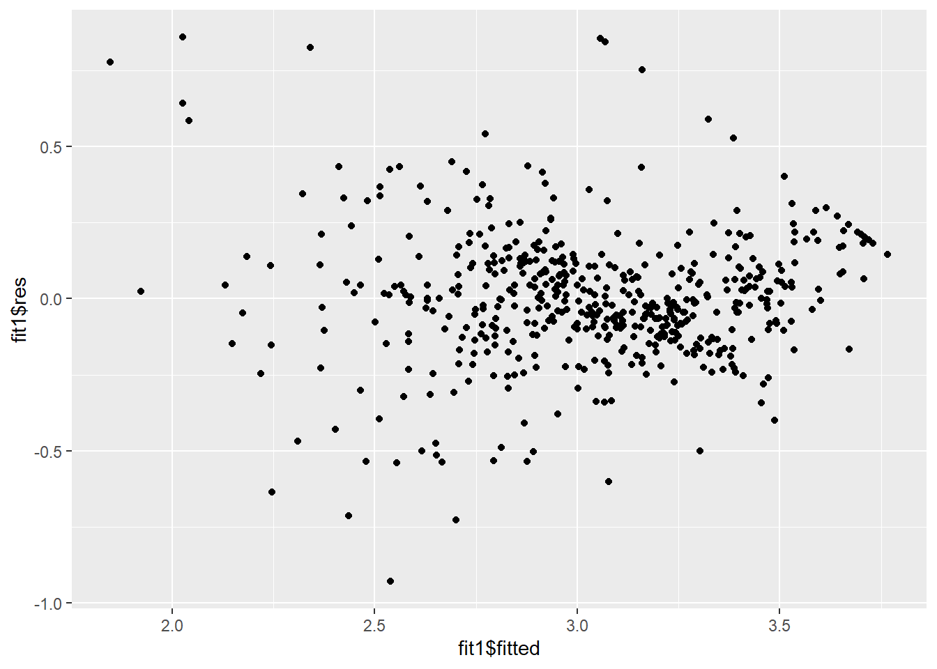

At a first glance, the residual plot shows us that the residual values seem to decrease as the fitted value increases, meaning that the model doesn’t fit the data very well, albeit not in a dramatic way. A well-built linear model should have the following traits in a fitted vs residuals plot:

1. The residuals “bounce randomly” around the zero-line, suggesting that the assumption that the relationship is linear is reasonable.
2. The residuals roughly form a “horizontal band” around the zero-line, suggesting the variances of the error terms are equal.
3. No residual stands out from the random residual pattern, suggesting there are no outliers.

The plot produced above does not possess the first and second qualities, forming a conal shape, rather than a horizonal band, while the residuals do not appear to take on a random pattern, instead becoming closer to the zero-line as the fitted values increase.

With this in mind, we can check out the initial correlation coefficients.

c(summary(fit1)$r.squared, summary(fit1)$adj.r.squared, AIC(fit1), BIC(fit1))

[1]   0.7143414   0.7126343 -94.4023297 -73.2696463

The All-Subsets algorithm

First things first, we’ll install a new package called leaps, by running install.packages('leaps'). The leaps package contains functions that allow us to perform an exhaustive search for the best subsets of variables in x to predict a variable y.

library(leaps)

Warning: package 'leaps' was built under R version 4.3.3

model.allsubset = regsubsets(log(medv) ~ lstat + rm + indus + tax + nox + ptratio, data = Boston)
summary(model.allsubset)

Subset selection object
Call: regsubsets.formula(log(medv) ~ lstat + rm + indus + tax + nox + 
    ptratio, data = Boston)
6 Variables  (and intercept)
        Forced in Forced out
lstat       FALSE      FALSE
rm          FALSE      FALSE
indus       FALSE      FALSE
tax         FALSE      FALSE
nox         FALSE      FALSE
ptratio     FALSE      FALSE
1 subsets of each size up to 6
Selection Algorithm: exhaustive
         lstat rm  indus tax nox ptratio
1  ( 1 ) "*"   " " " "   " " " " " "    
2  ( 1 ) "*"   " " " "   " " " " "*"    
3  ( 1 ) "*"   "*" " "   " " " " "*"    
4  ( 1 ) "*"   "*" " "   "*" " " "*"    
5  ( 1 ) "*"   "*" "*"   "*" " " "*"    
6  ( 1 ) "*"   "*" "*"   "*" "*" "*"    

Based on this output, we see that the optimal model with one variable is lstat, and the best model with three predictors uses lstat, rm, and ptratio. The number on each row represents a model with that number of predictors, while the * sign below predictors indicate that it’s included in the model.

The first row contains the best model with one predictor. The asterisk under lstat tells us that it’s the sole predictor.

Additionally, the summary() function works on objects from regsubsets(), meaning that we can identify values such as the R-squared, adjusted R-squared, and Cp of all the models shown above.

# Examining the models using R-squared criterion
summary(model.allsubset)$rsq

[1] 0.6480799 0.6948709 0.7143414 0.7241510 0.7255888 0.7269433

# Adjusted R-squared
summary(model.allsubset)$adjr2

[1] 0.6473817 0.6936576 0.7126343 0.7219486 0.7228447 0.7236601

# Cp
summary(model.allsubset)$cp 

[1] 141.119611  57.611109  24.029450   8.102819   7.475344   7.000000

Based on the R^2, adjusted R^2, and C_p values, the best model among all those presented in model.allsubset happens to be the last model, which includes all the given variables. We’ll denote that model as the fit2 model.

When basing the models off of the BIC score, the best model is the one with 4 predictors, lstat, rm, tax, and ptratio, and we’ll denote this model as fit3.

fit2 = lm(log(medv) ~ lstat + rm + indus + tax + nox + ptratio, data = Boston)
plot(fit2$res~fit2$fitted)
fit3 = lm(log(medv) ~ lstat + rm + tax + ptratio, data = Boston)
plot(fit3$res~fit3$fitted)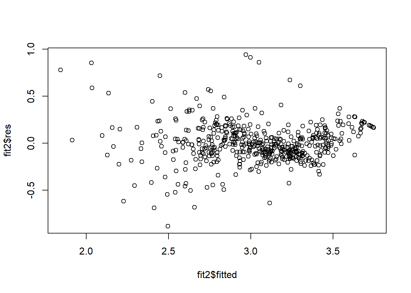

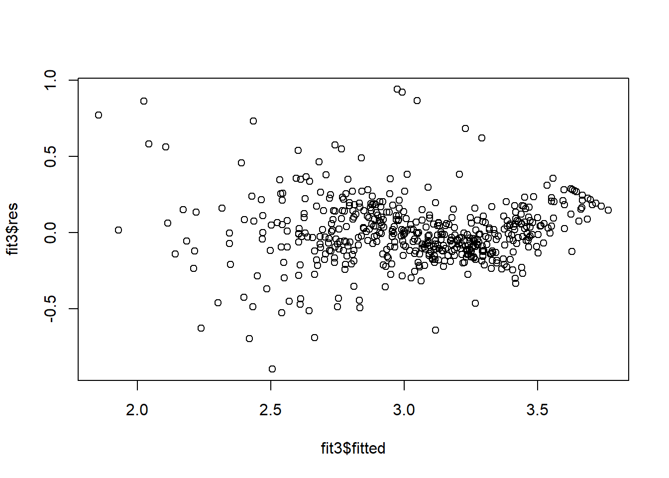
fit2 (log(medv) ~ lstat + rm + indus + tax + nox + ptratio)

fit3 (log(medv) ~ lstat + rm + tax + ptratio)

When comparing the residual plots for fit2 and fit3, we see a similar issue that the fit1 model had, where the residuals vs fitted plot appears to take on a conal shape instead of an evenly-distributed horizontal band. If this is the case, how do we tell which model is the best?

In this scenario, we’ll look at the models based on their AIC and BIC score.

res = matrix(0, nrow=3, ncol=4) # initiate a 3 by 3 matrix. 

colnames(res) = c("R-sq","adj R-sq", "AIC", "BIC")

res[1,] = c( summary(fit1)$r.squared, summary(fit1)$adj.r.squared,AIC(fit1),BIC(fit1) )
res[2,] = c( summary(fit2)$r.squared, summary(fit2)$adj.r.squared,AIC(fit2),BIC(fit2) )
res[3,] = c( summary(fit3)$r.squared, summary(fit3)$adj.r.squared,AIC(fit3),BIC(fit3) )

res

          R-sq  adj R-sq        AIC       BIC
[1,] 0.7143414 0.7126343  -94.40233 -73.26965
[2,] 0.7269433 0.7236601 -111.23199 -77.41970
[3,] 0.7241510 0.7219486 -110.08387 -84.72465

Results:

• fit2 is the best model when basing our judgement on R^2, adjusted R^2, and AIC.
• fit3 would be the best model when looking at the BIC score.

Model selection by Cross-Validation

When using the All-Subsets algorithm, we obtained a total of three models: fit1, fit2, and fit3. However, we had a difficult time determining which of the three models predicted medv the best. Now, we consider applying the Cross-Validation technique to the three models.

To do so, we’ll have to first install the DAAG package by running install.packages("DAAG").

library(DAAG)

# Initiate a vector to record the overall Mean Square Error (MSE) of each model
ms.vec = NULL 

First, we’ll run a 3-fold Cross-Validation for the fit1 model.

cv.res = CVlm(Boston, fit1, m=3)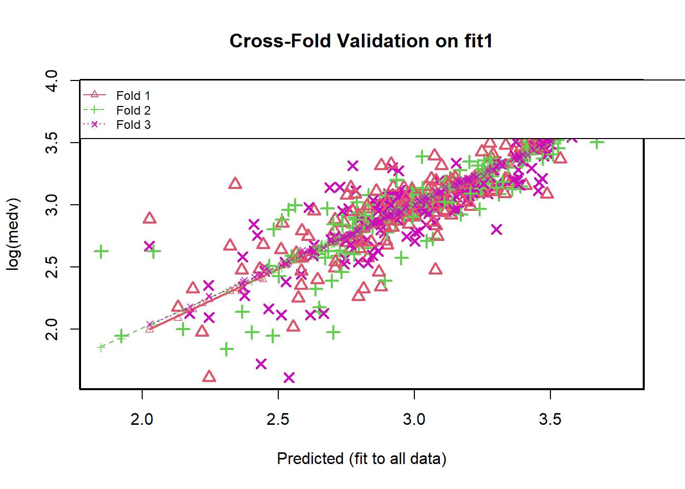

When running the above code, R will additionally print a lot of data from the CVlm() function, including the number of observations in each fold, the sum of squares value, and mean square.

The above code generates these results:

Fold #	Observations (n)	Sum of Square Error (SSE)	Mean Square Error (MSE)
1	168	8.82	0.05
2	169	7.3	0.04
3	169	8.64	0.05

To obtain the overall MSE value from all 3 folds, we run the code:

attr(cv.res, "ms") # prints the MSE value

[1] 0.04895046

ms.vec = c(ms.vec, attr(cv.res, "ms")) # create a vector to save the MSE values for each fit

Now we’ll run the CVlm() on fit2 and fit3 models for comparison.

cv.res2 = CVlm(Boston, fit3, m=3)
ms.vec = c(ms.vec, attr(cv.res2, "ms"))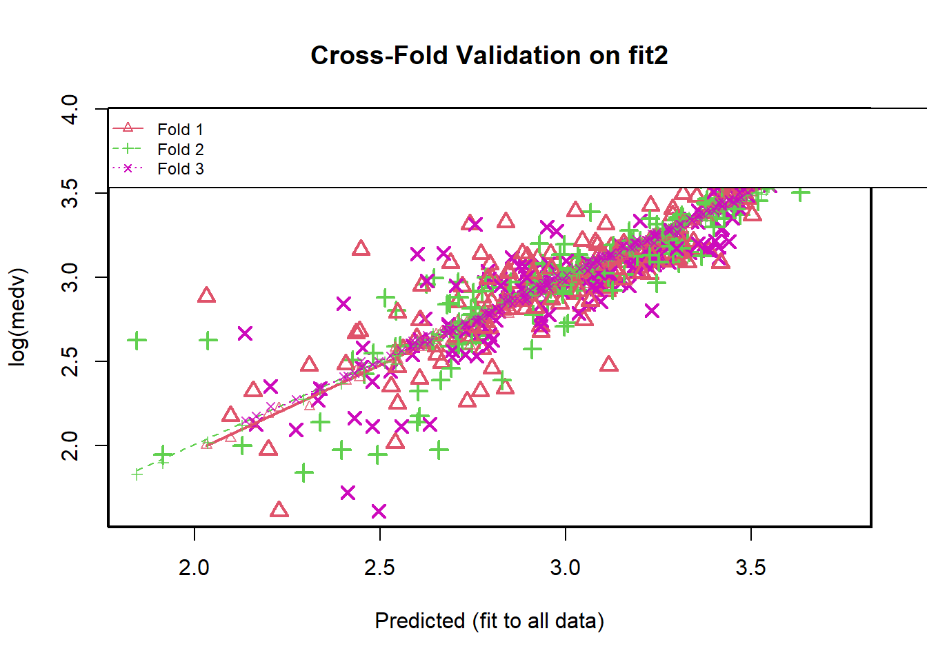

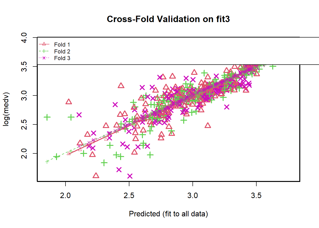
ms.vec

[1] 0.04895046 0.04768977 0.04776739

The overall MSE based on a 3-fold CV suggests that fit2 and fit3 are similar (0.0477 for fit2, and 0.0478 for fit3). Since a lower MSE score indicates a better fit, we can assume that fit1 is not the best fit.

Between fit2 and fit3, since their MSE values are close, we can use the Parsimony or KISS rule, which states that you should choose the explanation that uses the fewer assumptions (which in this case, uses the fewest predictors). When looking at the BIC values of each fit, it also suggests that fit3 is the best model.

summary(fit3)

Call:
lm(formula = log(medv) ~ lstat + rm + tax + ptratio, data = Boston)

Residuals:
     Min       1Q   Median       3Q      Max 
-0.89537 -0.11738 -0.01467  0.10071  0.93843 

Coefficients:
              Estimate Std. Error t value Pr(>|t|)    
(Intercept)  3.425e+00  1.639e-01  20.903  < 2e-16 ***
lstat       -3.169e-02  1.944e-03 -16.307  < 2e-16 ***
rm           1.140e-01  1.770e-02   6.442 2.77e-10 ***
tax         -3.059e-04  7.247e-05  -4.221 2.89e-05 ***
ptratio     -3.149e-02  5.172e-03  -6.090 2.25e-09 ***
---
Signif. codes:  0 '***' 0.001 '**' 0.01 '*' 0.05 '.' 0.1 ' ' 1

Residual standard error: 0.2155 on 501 degrees of freedom
Multiple R-squared:  0.7242,    Adjusted R-squared:  0.7219 
F-statistic: 328.8 on 4 and 501 DF,  p-value: < 2.2e-16

fit2 (log(medv) ~ lstat + rm + indus + tax + nox + ptratio) fit3 (log(medv) ~ lstat + rm + tax + ptratio)