Hierarchical Clustering

In this lab section, we’ll learn how to apply the hierarchical clustering algorithm to the Iris dataset.

Hierarchical clustering is an alternative approach to the clustering we know of, which does not need us to commit to a particular choice of k.

There are two common types of hierarchical clustering, bottom-up method, and the agglomerative method, which will be covered in the lab.

Hierarchical Clustering using all Variables

In the K-Means chapter, we were required to specify the number of clusters prior to building the model, and finding the optimal number of clusters can often be pretty hard! Hierarchical clustering gives us the ease of running a model without having to worry about whether or not the k value is optimized.

The algorithm works as follows:

Put each data point in its own cluster.
Identify the closest two clusters and combine them into one cluster.
Repeat step two until all the data points are in a single cluster.
Once this is done, it is usually represented by a dendrogram-like structure.

Visualization of the clustering process (Bock, T. DisplayR.) — Visualization of the clustering process (Bock, T. *DisplayR*.)

There are a few ways to determine how close two clusters are:

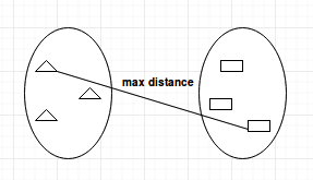
Complete-linkage

The complete-linkage method finds the maximum possible distance between points belonging to two different clusters before merging. This means that the distance between two clusters is measured by the furthest distance between two points.

This method will identify the smallest minimum distance between two clusters and merge them together.

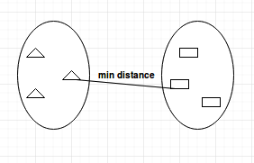
Single-linkage

The single-linkage method works oppositely of complete-linkage. This method finds the shortest distance between points belonging to two different clusters. This means that the distance between two clusters is measured by the shortest distance between two points.

This method will identify the smallest minimum distance between two clusters and merge them together.

Average-linkage

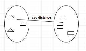
The average-linkage method calculates all possible pairwise distances for points belonging to two different clusters and then calculates the average of all the distances. This means that the distance between two clusters is measured by the average distance between all possible pairs of points.

This method will identify the average distance between two clusters and merge them together.

Centroid-linkage

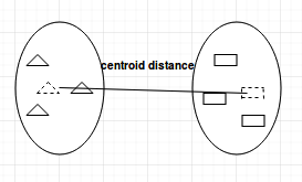
The centroid-linkage method calculates the centroid of every cluster (the mean location between every point in a cluster). This means the distance between means of two clusters is how distance is measured.

This method will identify the distance between two cluster means and merge them together.

The hclust package

To see how well the hierarchical clustering algorithm performs, we’ll use the hclust() function, which should be installed in R by default (if it isn’t, the command install.packages("stats") should do the trick).

This package requires us to provide the data in the form of a distance matrix, which is achievable using the dist() function. By default, hclust() uses the complete-linkage method.

# Prepare the data without the class (iris species) information 
iris.unclass = iris[,c(1,2,3,4)]
iris.class = iris[,"Species"]
head(iris.unclass)

Sepal.Length	Sepal.Width	Petal.Length	Petal.Width
5.1	3.5	1.4	0.2
4.9	3.0	1.4	0.2
4.7	3.2	1.3	0.2
4.6	3.1	1.5	0.2
5.0	3.6	1.4	0.2
5.4	3.9	1.7	0.4

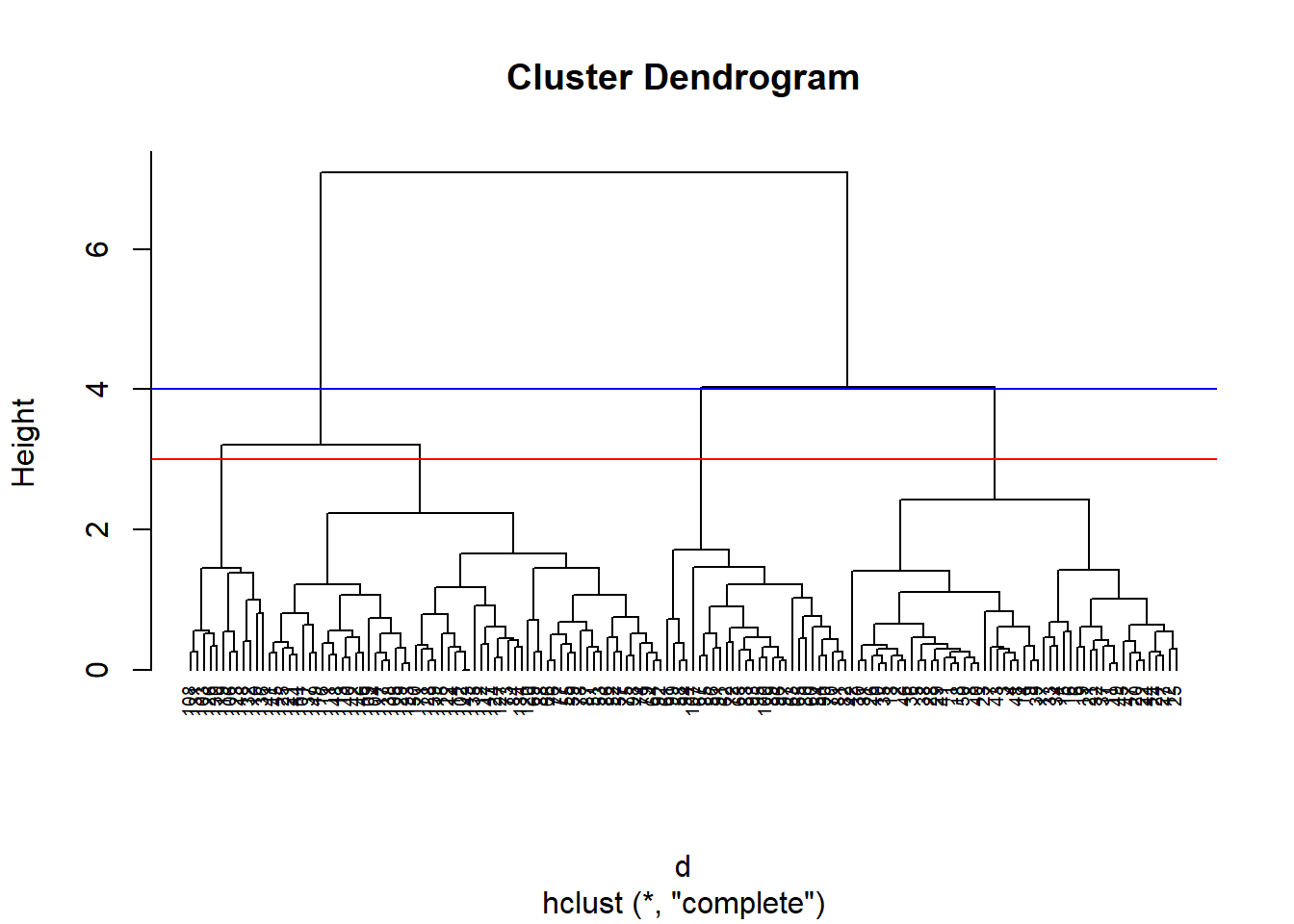
set.seed(311)
# Dissimilarity matrix
d = dist(iris.unclass, method = "euclidean")

# Hierarchical clustering using Complete Linkage
hc.comp = hclust(d, method = "complete" )

# Plot the obtained dendrogram
plot(hc.comp, cex = 0.6, hang = -1)
# Display cuts at dendrogram height 3 and 4
abline(h =c(3,4),col = c('red','blue'))

In the plot above, we’ve plotted two different cuts, one where the height = 4, and one where the height = 3. The number of clusters we end up with depends on where we cut the dendrogram.

If we cut the dendrogram where the height is equal to four, we’ll end up with three distinct clusters, since the line cuts through three branches.
If we cut the dendrogram where the height is equal to three, we’ll end up with four clusters, since the line cuts through four branches.

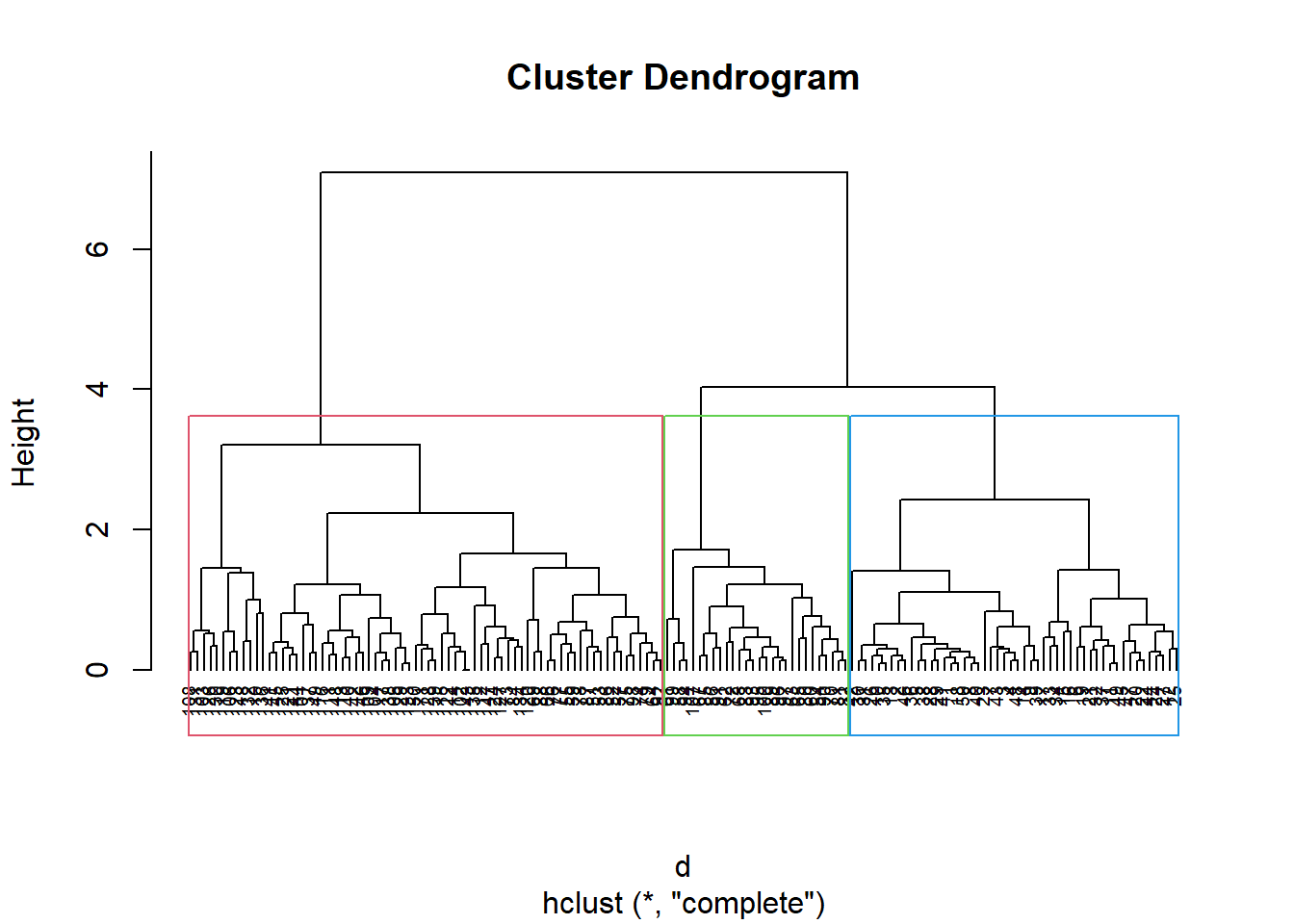
Let’s go ahead and separate the dendrogram into three clusters visually, which would be the equivalent of making a cut at height = 4:

plot(hc.comp,cex=0.6,hang=-2)
rect.hclust(hc.comp , k = 3, border = 2:4)

We can see that if we cut off the height at four, we’ll end up with three distinct branches, each one in their own coloured box.

Since cluster analysis is an exploratory approach, there is no definitive answer as to whether or not we should be making the cut at height = 3 or height = 4 since the answer is often extremely context-dependent. In cluster validation, the most common method of comparing cluster numbers is demonstrated (using silhouette width).

For now, we’ll go ahead and tell R that we want three clusters. To do this, we’ll cut off the tree at the desired number of clusters using cutree()

clusterCut = cutree(hc.comp, 3)
# Now let us compare with original labels
table(clusterCut, iris.class)

clusterCut	setosa	versicolor	virginica
1	50	0	0
2	0	23	49
3	0	27	1

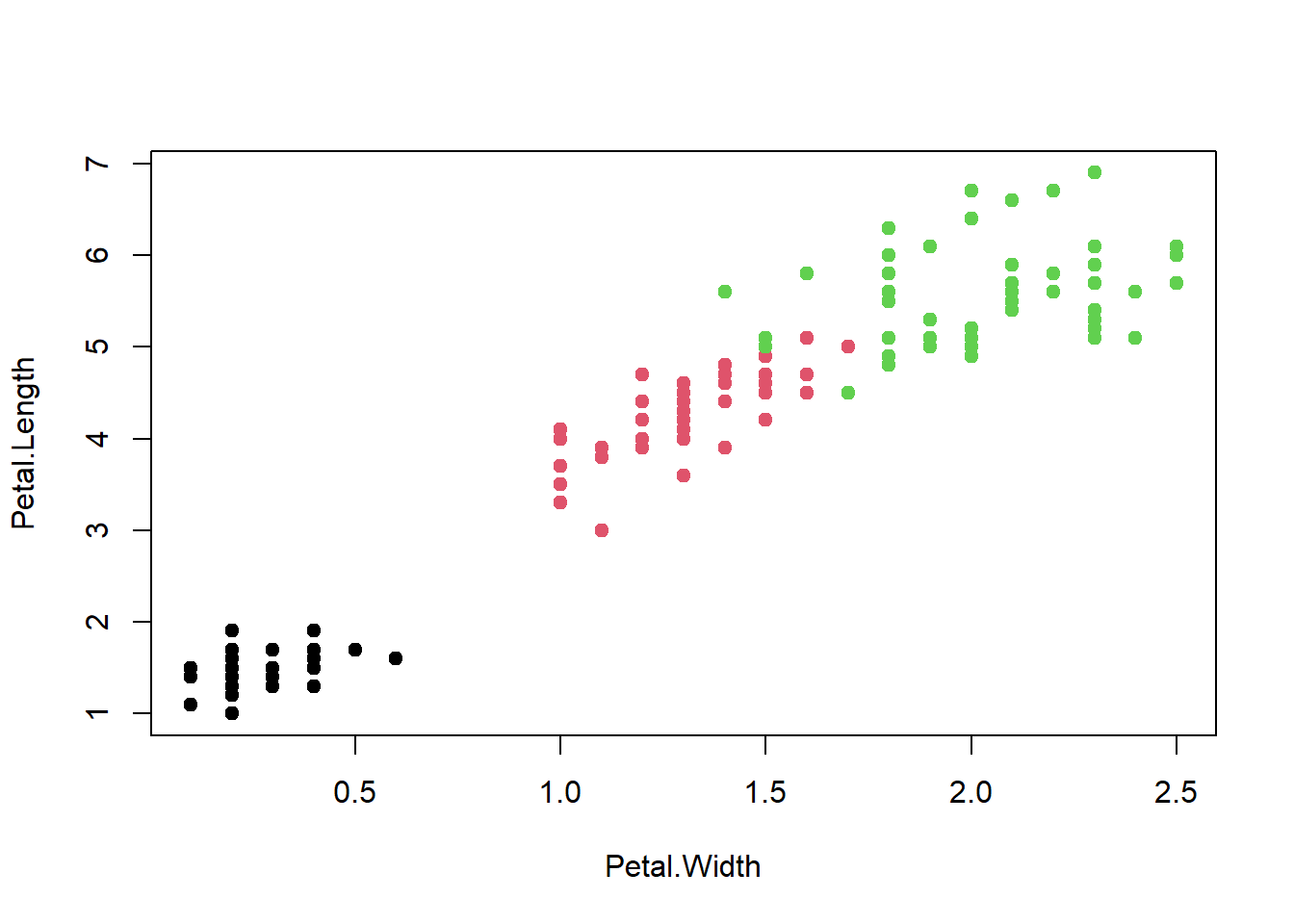
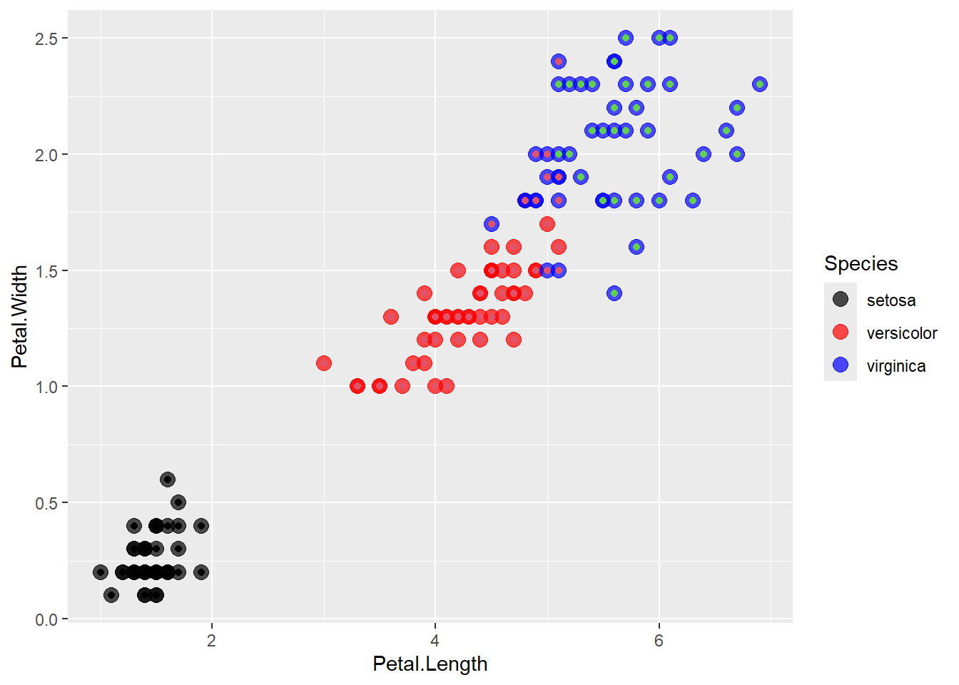
It looks like the algorithm successfully classified all the flowers of species setosa into cluster 1, and most virginica into cluster 2, but had trouble with versicolor. If you look at the original plot showing the different species, you can understand why:

plot(Petal.Length~Petal.Width, data=iris.unclass, col=iris.class,pch=19)

When plotting out Petal.Length and Petal.Width on a graph, we see that the red cluster and green cluster are quite close to each other (which is likely where the versicolor and virginica misclassifications occurred).

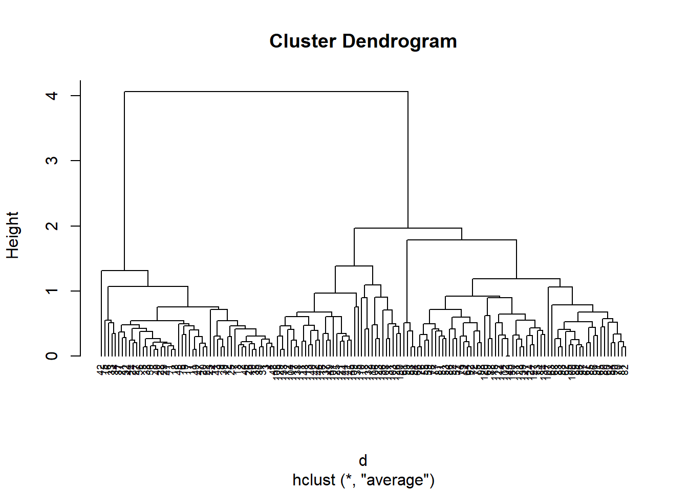
Let’s see if we can improve this by using a different linkage method. This time we’ll use the mean-linkage method shown in the average-linkage method:

hc.avg = hclust(d, method = 'average')
plot(hc.avg, cex = 0.6, hang = -1)

Here, we see that either having 3 or 5 clusters are the best choices. Let’s use cutree() to bring it down to 3.

cut3 = cutree(hc.avg, 3)
table(cut3, iris.class)

setosa	versicolor	virginica
50	0	0
0	50	14
0	0	36

We can see that this time, the algorithm did a much better job of clustering the data, having slight difficulty classifiying the virginica species, though overall a much cleaner classification compared to the first attempt.

We can plot it using ggplot2 as follows to compare it with the original data:

library(ggplot2)
ggplot(iris, aes(Petal.Length, Petal.Width, color =Species))+  
   geom_point(alpha = 0.7, size = 3.5) + geom_point(col = cut3)+
   scale_color_manual(values = c('black', 'red', 'blue'))

All the points where the inner color doesn’t match the border color are the ones which were classified/clustered incorrectly.

Estimating the Number of Clusters

We won’t always have the labelled data like we do for the iris dataset. If we wanted to know the exact number of classes, there’s different criteria involved in estimating it. Some of these methods you may already be familiar with from clustering estimating in the K-Means chapter.

Elbow method

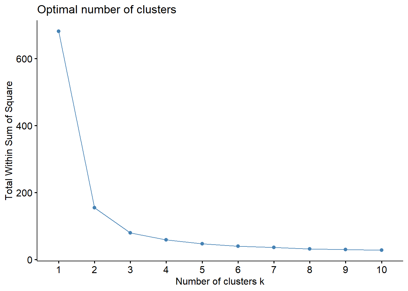
We’ve already demonstrated the elbow method in the K-Means chapter, however, this time, we’ll try applying it to the iris dataset and see what we get.

# From the factoextra library
fviz_nbclust(iris.unclass, FUN = hcut, method = "wss")

In this graph, we see that the elbow is approximately at k = 3, since that is where the total within sum of squares value stops decreasing as drastically!

Average silhouette method

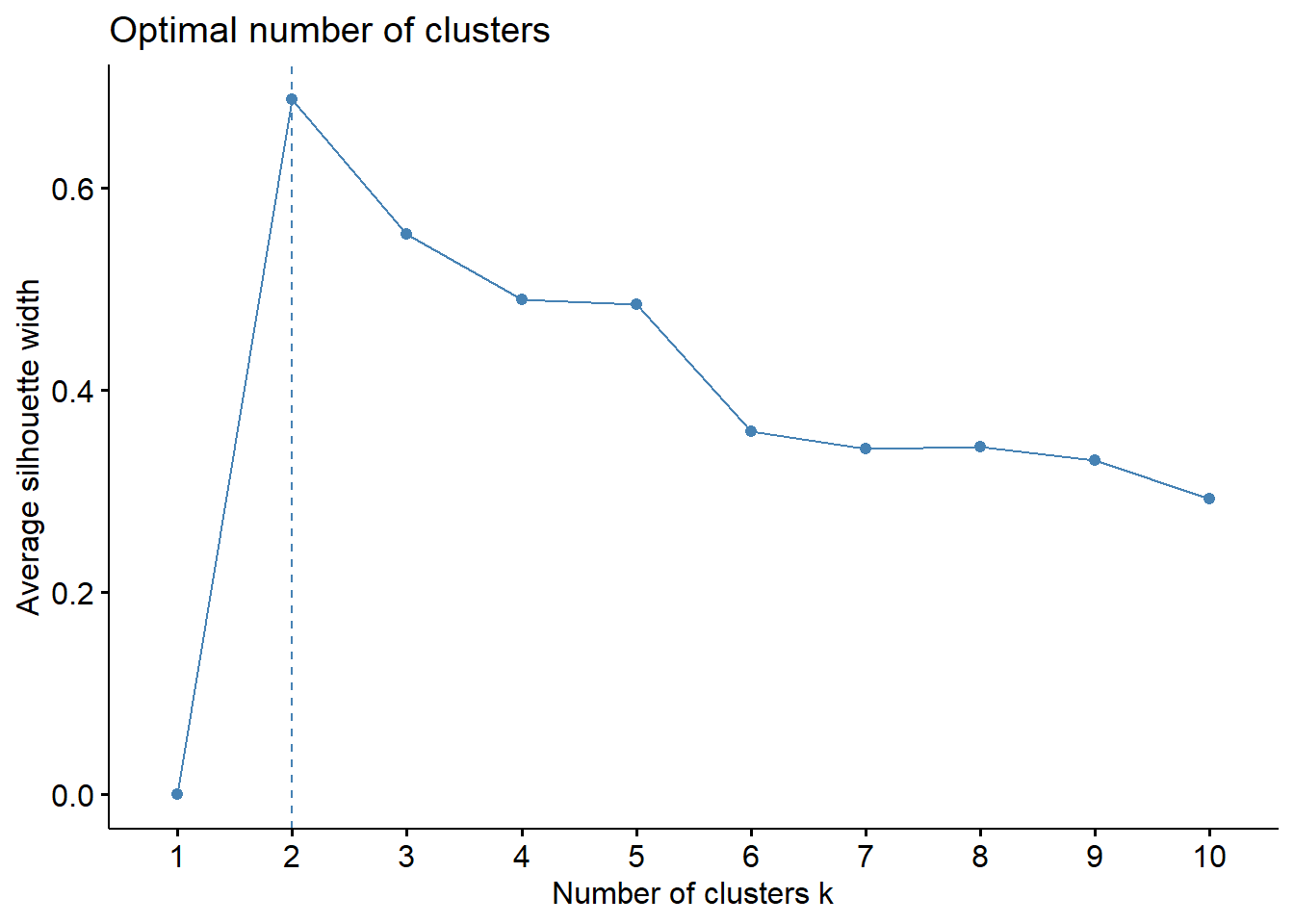
We’ve also demonstrated the silhouette method in the K-Means chapter. We’ll run again this time in the context of the iris dataset!

fviz_nbclust(iris.unclass, FUN = hcut, method = "silhouette")

Gap statistic method

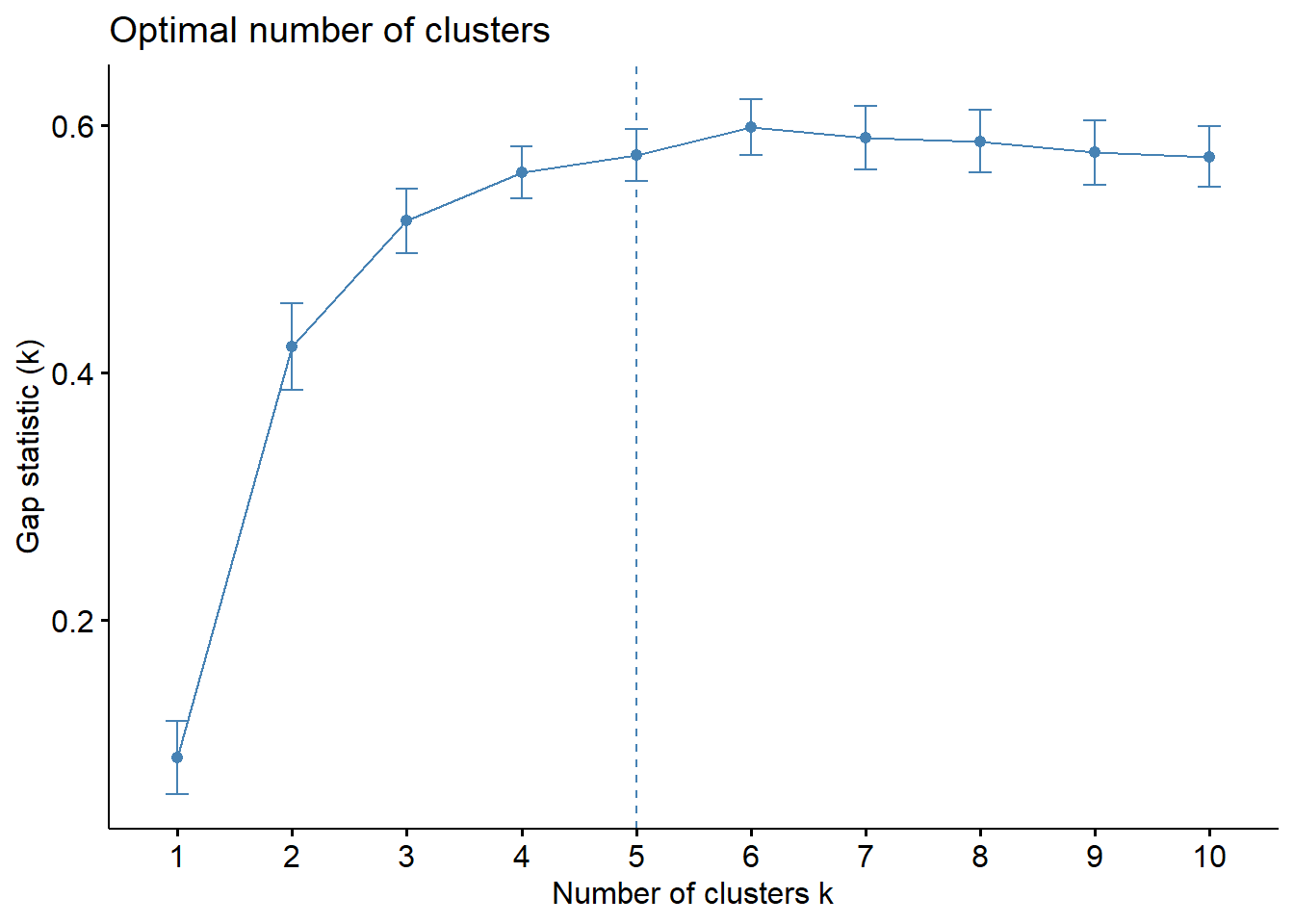
The gap statistic method was not covered in the previous sections, this one is new! It selects the number of clusters by comparing the total intravluster variation for different values of k. The optimal k it finds is the value that yields the largest gap statistic.

# The function is from the cluster library
gap_stat = clusGap(iris.unclass, FUN = hcut, nstart = 25, K.max = 10, B = 50)
fviz_gap_stat(gap_stat)

Additional Comments

Clustering can be a very useful tool for data analysis in the unsupervised setting. However, there’s a number of issues that arise when we perform clustering. In the context of hierarchical clustering, we should worry about:

What dissimilarity measure should we use? The choice of distance measure is very important, and has a strong effect on the clustering results. (Pay attention to the type of data we’re clustering and the question we want to answer!)
What kind of linkage should be used? Generally, centroid-linkage or average-linkage provides balanced results, though we should still take the context of the data into comparison.
Where should we cut the dendrogram in order to obtain clusters? This is a difficult question when we don’t know the k value. There’s many algorithms that attempt to calculate the optimal location to cut it, however, sometimes the most reliable way is to test it ourselves and compare the results at different cuts!

Each of these decisions can have a strong impact on the results obtained. In practice, we’ll try several different solutions, and look for the one with the most useful or interpretable results. With these methods, there is no single right answer - any solution that exposes some interesting aspects of the data should be considered.