K-Nearest Neighbours

In a K-nearest Neighbours (KNN) classification, a sample point is classified based on the majority votes of its K-nearest neighbours in the training data.

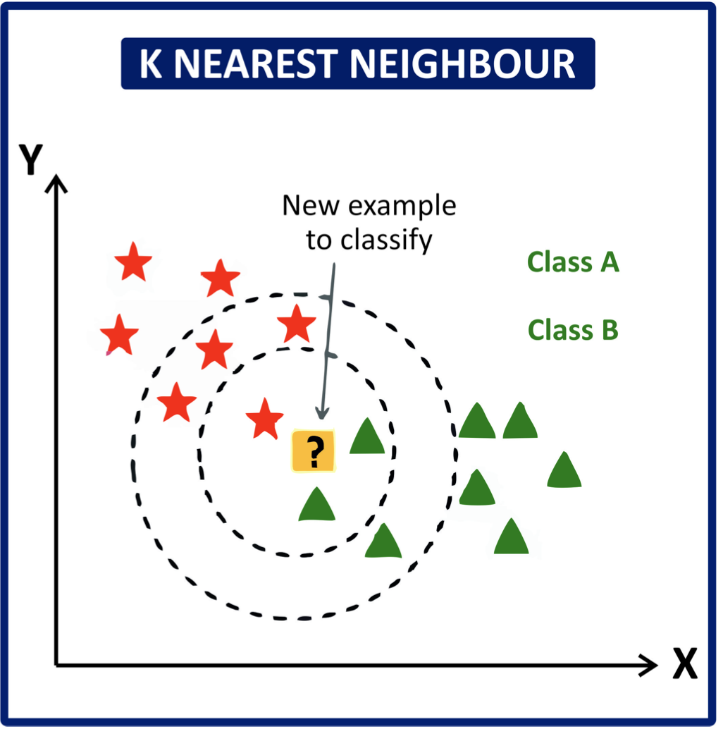
kNN example (Al-Serw, N. 2021. Analytics Vidhya.) — kNN example (Al-Serw, N. 2021. *Analytics Vidhya*.)

In the image above, the innermost circle considers the three closest neighbours. In that case, there are two green triangles and one red star, considering the majority vote goes to the green triangles, the sample point is also classified as a green triangle. The outer circle counts the circles inside it as well, taking votes from the nearest seven neighbours. In this case, there are four red stars and three green triangles, and the model would classify the sample point as a red star.

Depending on the specified number of neighbours the model will take into account, the resulting classification may differ.

Introduction to the Credit Card Dataset

In this lab, we’ll explore the applications of K-nearest Neighbours using an exercise as an example. For the task, we are interested in predicting whether an individual will default on their credit card payment, on the basis of annual income and monthly credit card balance. We’ll build a kNN classifier to achieve this task.

Each data point we train the model on will have these variables:

Default: factor (yes, no)
Student: factor (yes, no)
Balance: numerical variable - monthly credit card balance.
Income: numerical variable - annual income.

Below is the Default (credit card) dataset output, when calling the first few rows of it, and summarizing each variable in R.

# install.packages("ISLR")
# install.packages("class")

library(ISLR)
library(class)
head(Default)

default	student	balance	income
No	No	729.5265	44361.625
No	Yes	817.1804	12106.135
No	No	1073.5492	31767.139
No	No	529.2506	35704.494
No	No	785.6559	38463.496
No	Yes	919.5885	7491.559

str(Default)

'data.frame':   10000 obs. of  4 variables:
 $ default: Factor w/ 2 levels "No","Yes": 1 1 1 1 1 1 1 1 1 1 ...
 $ student: Factor w/ 2 levels "No","Yes": 1 2 1 1 1 2 1 2 1 1 ...
 $ balance: num  730 817 1074 529 786 ...
 $ income : num  44362 12106 31767 35704 38463 ...

An Analysis of the Credit Card Dataset

Now let us find the proportion of defaulters and students in this dataset.

# Returns the proportion of defaulters in the 'yes' category
table(Default$default)/nrow(Default)


    No    Yes 
0.9667 0.0333

# Returns number of students with and without a default
table(Default$student)


  No  Yes 
7056 2944

# Returns the number of students who do not have credit card defaults
sum(Default$student == "Yes" & Default$default == "No")

[1] 2817

# The yes/no rows shows default status, the yes/no columns shows student status
table(Default$default,Default$student)

     
        No  Yes
  No  6850 2817
  Yes  206  127

From the above outputs, we can surmise that in this dataset, about 3.33% of credit cards are defaulters and approximately 29.44% credit accounts belong to students.

To look into this further, below, the data is separated to calculate the default rate for students and non-students.

127/(2817+127) # Default rate in students

[1] 0.04313859

206/(6850+206) # Default rate in non-students

[1] 0.02919501

The calculation above suggests that the students have a higher default rate (students have a 4.32% chance of defaulting, while non-students have a 2.92% chance). From looking at this, we know that whether or not a credit account is owned by a student is a key predictor to prediction default-status.

We can also compare the numerical differences in variables like balance by looking at a boxplot:

boxplot(balance~default,data=Default,col="lightblue")
boxplot(income~default,data=Default,col="lightpink")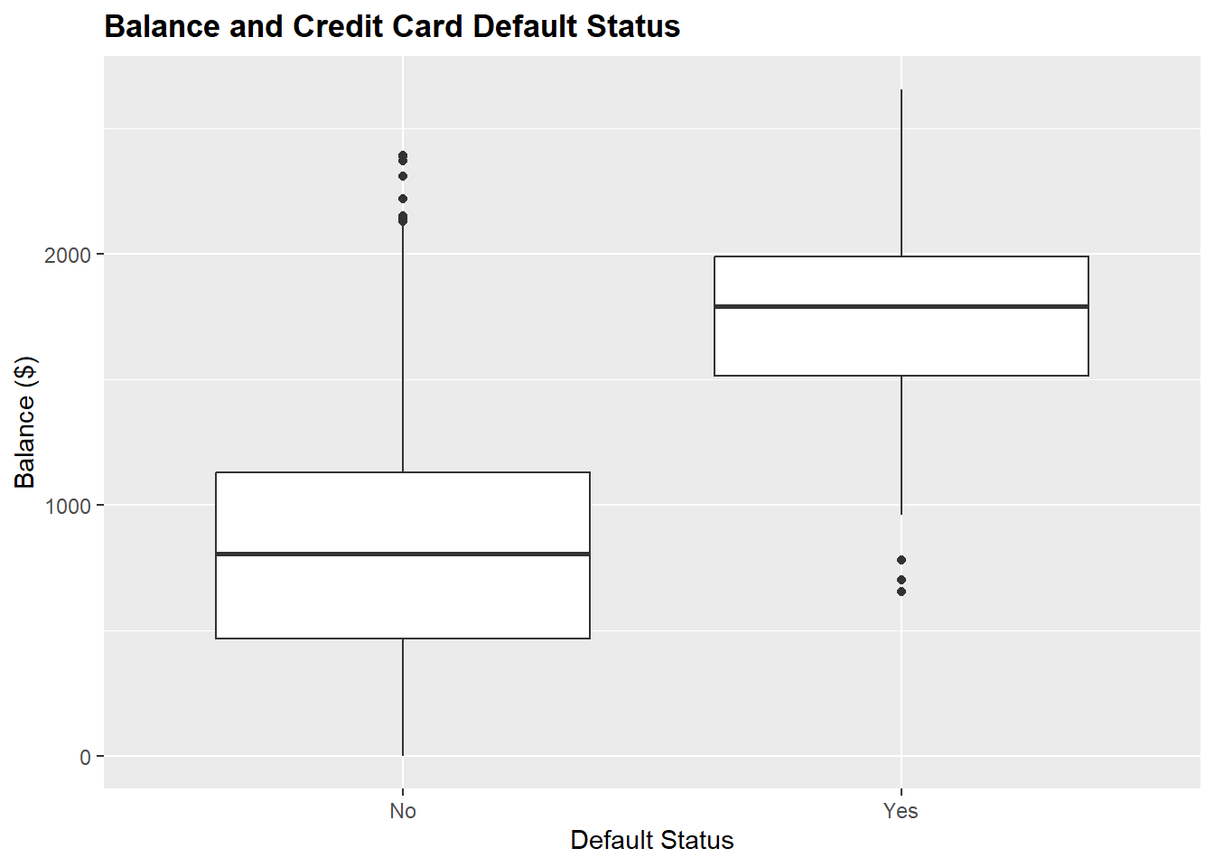

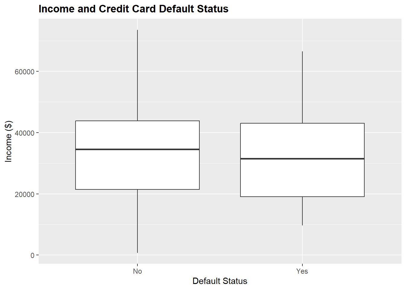
The boxplots show a drastic difference in balance numbers between defaulted credit cards and non-defaulted ones. Alongside the student status, balance could be an important predictor for defaulting.

Training the KNN classification model

To perform KNN for classification, we will use the knn() function included in the class package.

From the lectures, we know that knn() requires all predictors to be numeric, which some of our variables don’t follow. To fix this, we’ll coerce student to be a binary variable where ‘yes’ = 1, and ‘no’ = 0.

We can, and should leave the response variable, default, as a factor in classification models.

# We minus one from the output of as.numeric()
# This is because as.numeric() when applied on factors will start from 1
Default$student = as.numeric(Default$student) - 1

Before a classification model is ready to test on data, it first must be trained on a sample dataset. We can achieve this by splitting the data in Default randomly into separate testing and training sets.

The testing set evaluates the model after it is built. The training set is what the KNN model uses for the nearest-neighbour votes.

set.seed(42)

## Split the data into training and testing set
default_idx = sample(nrow(Default), 5000) 
default_trn = Default[default_idx, ] 
default_tst = Default[-default_idx, ]

# Training data
x_train = default_trn[, -1] 
y_train = default_trn$default

# Testing data
x_test = default_tst[, -1] 
y_test = default_tst$default

Recall that defaulters are the minority class. The majority are non-defaulters. Before we move on,we should check the distribution of default in the training and testing dataset, a similar distribution is better.

table(y_train)/nrow(default_trn) # default distrn in training set

y_train
   No   Yes 
0.966 0.034

table(y_test)/nrow(default_tst) # default distrn in testing set

y_test
    No    Yes 
0.9674 0.0326

There is very little “training” when building KNN models. Essentially, the only training the model does is to simply remember the inputted data. Due to this, the KNN classifier has a very fast training time. However, when testing, the KNN classifier is very slow since for each test observation, the model must compute which points are the nearest neighbours.

Note that by default, knn() uses the Euclidean distance method to determine nearest neighbours.

head(knn(train = x_train, 
         test = x_test,
         cl = y_train, 
         k =3)
     )

[1] No No No No No No
Levels: No Yes

Here, knn() takes four arguments:

train: the predictors for the train set.
test:: the predictors for the test set. knn() will output classifications for each datapoint in this set.
cl: the true label classifications for the training set.
k: the number of neighbours to consider.

Testing the KNN Model

To evaluate the performance of the knn() model, we’ll create a function called find_class_err() to compare the success rate our model has in correctly classifying points in the test set.

find_class_err = function(actual, predicted) { 
  mean(actual != predicted)
}

Now that the evaluation function is created, we can go ahead and test our knn() model.

predict = knn(train = x_train, 
              test = x_test,
              cl = y_train,
              k = 3) 
find_class_err(actual = y_test, predict)

[1] 0.0344

The printed output shows a 3.18% accuracy rate in our current model. While this performance isn’t bad, we can improve on it by considering the scale of the predictor variables.

This is important because knn() relies on distance as a measure of the nearest neighbours, and our predictor variables scale off of different ranges of numerical values (0-1 for student compared to the large annual income numbers have a huge difference in the distance influence between each point.)

Often with knn() we need to consider the scale of the predictors variables. If one variable is contains much larger numbers because of the units or range of the variable, it will dominate other variables in the distance measurements. But this doesn’t necessarily mean that it should be such an important variable. It is common practice to scale the predictors to have a mean of zero and unit variance. Be sure to apply the scaling to both the train and test data

predict = knn(train = scale( x_train), 
              test = scale(x_test),
              cl = y_train,
              k = 3) 
find_class_err(actual = y_test, predict)

[1] 0.0318

Here we see the scaling slightly improves the classification accuracy. This may not always be the case, and often, it is normal to attempt classification with and without scaling.

Choosing the Correct k Parameter

How do we choose k? What is the number of nearest neighbours we should be looking at? Well, there isn’t one robust answer here, other than to try different values and see what works best!

For example, here’s a model with the k parameter set to 77:

pred = knn(train = scale(x_train), 
           test = scale(x_test),
           cl = y_train,
           k = 77) 
find_class_err(y_test, pred)

[1] 0.031

We can repeat the above process over all possible k values, and record the score for each k value.

set.seed(310)

# List all the k values to try
k_to_try = seq(1, by = 2, len = 50)

# Store all the error rates in the err_k vector
err_k = rep(x = 0, times = length(k_to_try))

# Execute the process using a for-loop 
for (i in 1:length(k_to_try)) { 

    pred = knn(train = scale(x_train), 
               test = scale(x_test), 
               cl = y_train,
               k = k_to_try[i])

    err_k[i] = find_class_err(y_test, pred) }

# Plot the results for the different k-values
plot(k_to_try, err_k, type = "b", col = "dodgerblue", cex = 1, 
     pch = 20, xlab = "k, number of neighbors", 
     ylab = "classification error", main = "(Test) Error Rate vs k Neighbors")

# Add line for min error seen
abline(h = min(err_k), col = "red", lty = 3)

# Add line for minority prevalence in test set
abline(h = mean(y_test == "Yes"), col = "grey", lty = 2)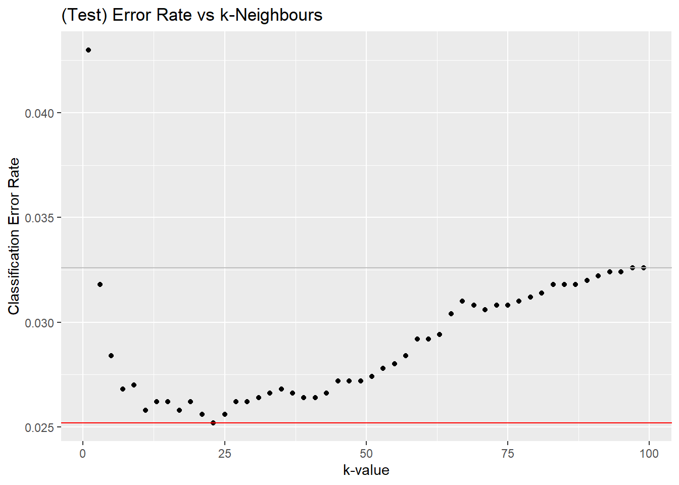

To manually output the optimal value in R, we can use min() on err_k to filter for the lowest value:

bestk = k_to_try[err_k == min(err_k)]
bestk

[1] 23

Now that we’ve found the best k-value to use, we fit the KNN model with bestk and get the error rate on the testing set.

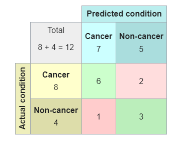
Using table(), we’ll also output a confusion matrix, which compares the actual values with the predicted values. Below is an example taken from wikipedia of a cancer prediction model:

pred = knn(train = scale(x_train), 
           test = scale(x_test),
           cl = y_train,
           k = bestk) 

table(y_test,pred) # confusion matrix

      pred
y_test   No  Yes
   No  4824   13
   Yes  113   50

find_class_err(y_test, pred) # find error rate on testing set

[1] 0.0252

We see here that after finding the optimal k-value, we are able to further minimize the error rate in our KNN model.

Using the Caret Package

The caret package allows us to easily calculate performance values given a vector of test data and a classification mode. It’ll output the accuracy rate, as well as the 95% confidence interval for the accuracy rate, as well as many other specifications.

To begin, we’ll start by loading the package in

# install.packages("caret")
library(caret)

Now we’ll use the confusionMatrix() function that comes with caret to calculate the performance values.

confusionMatrix(pred, y_test)

Confusion Matrix and Statistics

          Reference
Prediction   No  Yes
       No  4824  113
       Yes   13   50
                                         
               Accuracy : 0.9748         
                 95% CI : (0.9701, 0.979)
    No Information Rate : 0.9674         
    P-Value [Acc > NIR] : 0.001307       
                                         
                  Kappa : 0.4322         
                                         
 Mcnemar's Test P-Value : < 2.2e-16      
                                         
            Sensitivity : 0.9973         
            Specificity : 0.3067         
         Pos Pred Value : 0.9771         
         Neg Pred Value : 0.7937         
             Prevalence : 0.9674         
         Detection Rate : 0.9648         
   Detection Prevalence : 0.9874         
      Balanced Accuracy : 0.6520         
                                         
       'Positive' Class : No

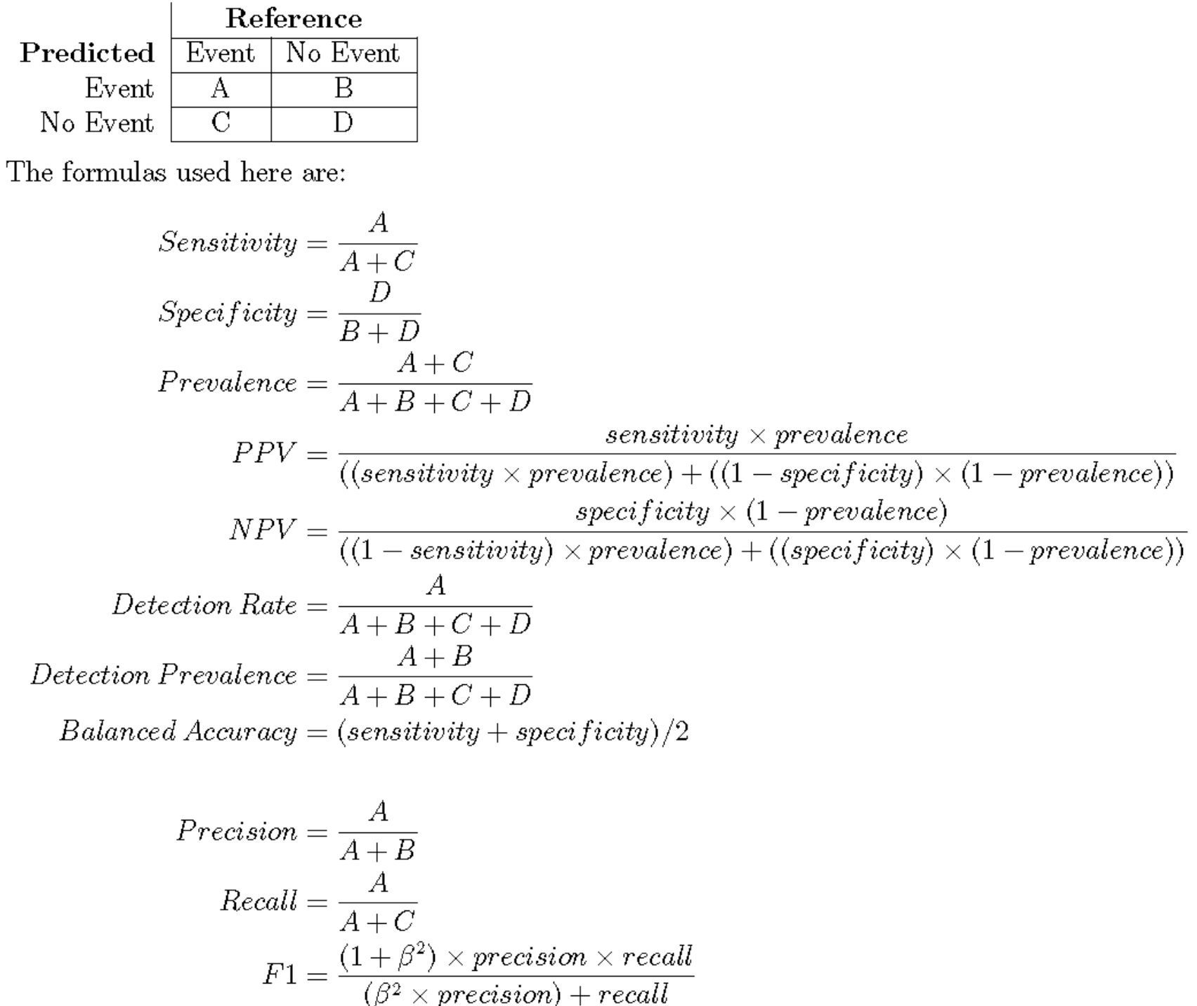
Below is the formula used for the performance value calculations for cross-referencing: