Regression trees are an important subtype of decision tree models that allow us to predict continuous, valued outputs. By design, they’re similar to classification trees, where they both use a decision tree-like algorithm.
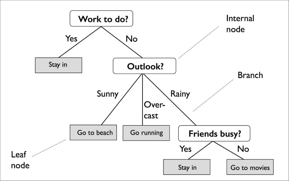
Regression tree example with categorical predictors (Li, L. 2019. Towards Data Science.)
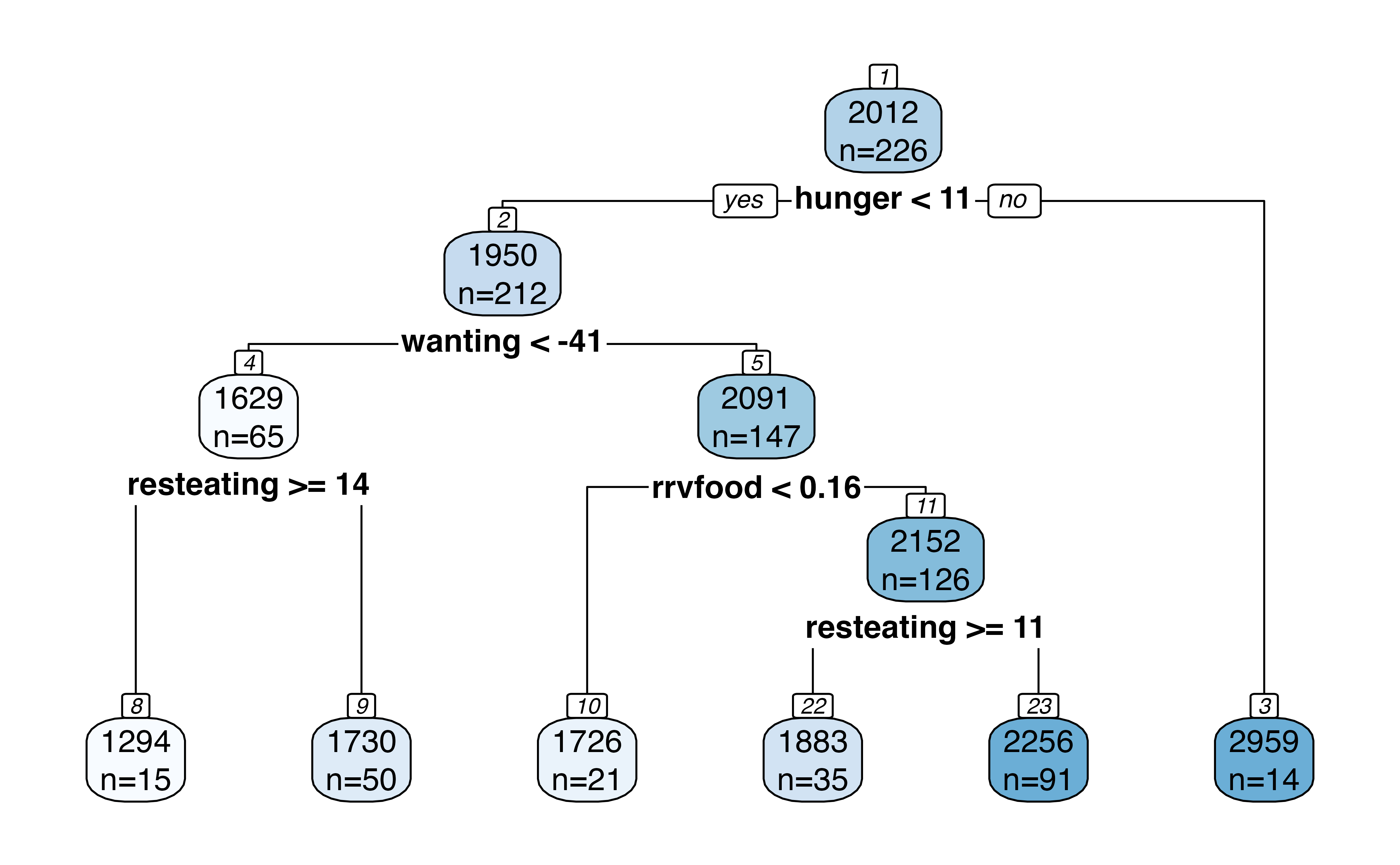
Regression tree example with numerical predictors (Neufield, A. Treevalues.)
In this chapter, we’ll explore both how to build an individual regression tree, as well as ensemble tree methods, which utilize multiple regression trees in its algorithm.
Below, are the summaries of each concept in this chapter:
Decision Tree: a hierarchical tree that models a set of decisions and their possible outcomes. Each decision is a conditional statement, based on a feature (variable) in the model.
Regression Tree: a decision tree that attempts to predict the final value of a continuous variable (non-categorical).
Pruning: a technique that cuts off parts of a decision tree, preventing it from growing too large and thusly overfitting the data.
Ensemble Tree: combines multiple decision trees together to make better predictions.
Random Forest: introduces variation in ensemble models by randomizing the features (variables) used in each tree.
Bagging: introduces variation in ensemble models by creating randomized subsets of the training data for each tree.
Data Preparation
To demonstrate regression trees, we’ll start by using the dataset from the Boston housing dataset, and recall that medv is the response variable we want to predict.
To start, we’ll split the data in half for the testing and training subsets.
To create our regression tree, we’ll start by loading in the tree library, which comes with the tree() function, taking in parameters in a similar format to lm().
# install.packages("tree")library(tree)atree =tree(medv ~ ., data = train) # A "." tells R to use all the featuressummary(atree)
Regression tree:
tree(formula = medv ~ ., data = train)
Variables actually used in tree construction:
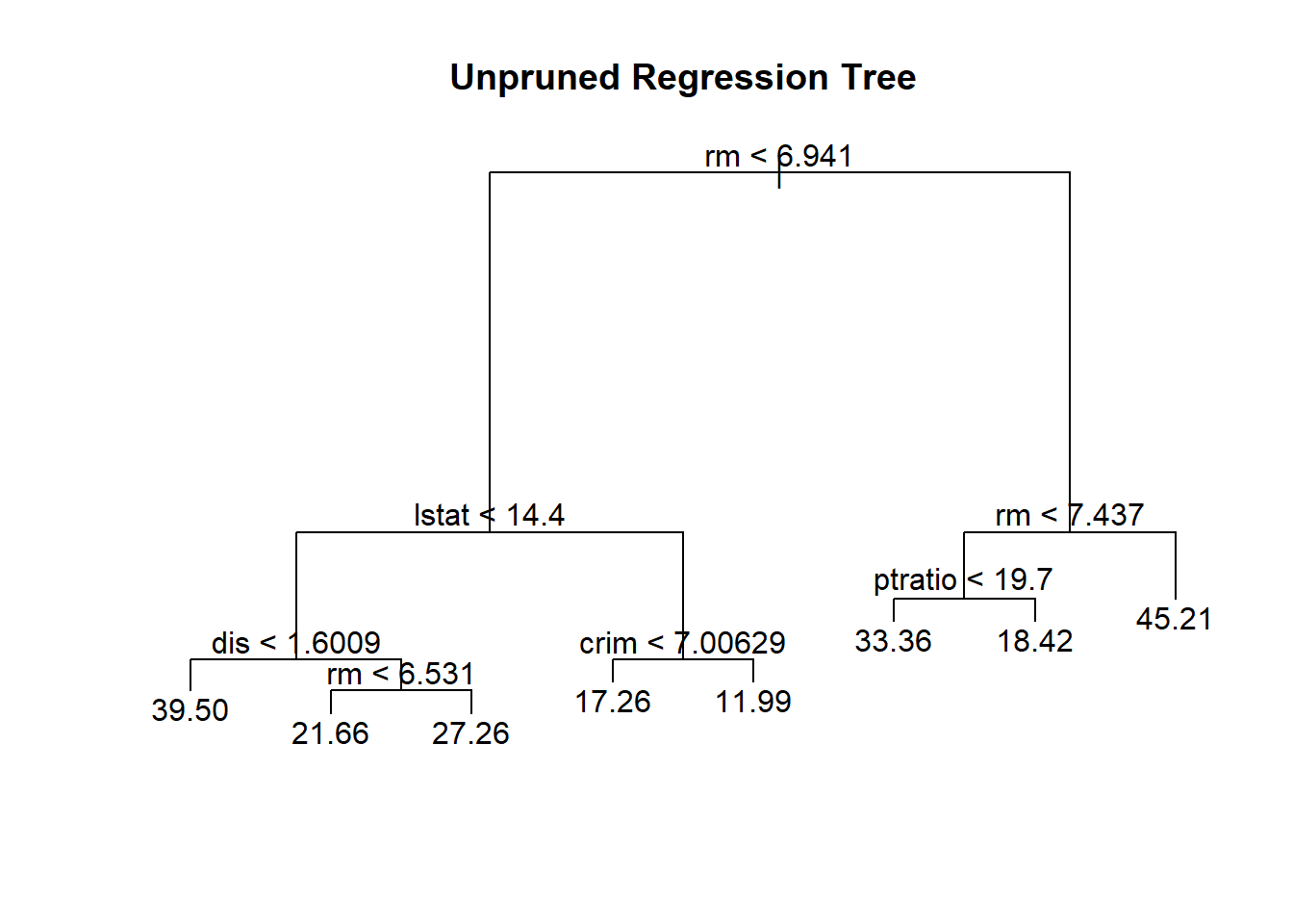
[1] "rm"      "lstat"   "dis"     "crim"    "ptratio"
Number of terminal nodes:  8
Residual mean deviance:  14.42 = 5712 / 396
Distribution of residuals:
     Min.   1st Qu.    Median      Mean   3rd Qu.      Max.
-23.31000  -2.07400   0.03691   0.00000   2.14300  14.54000
The summary() function when called on a tree object, lists the variables that are used as internal nodes in the tree, the number of terminal nodes, and the error rate on the training dataset.
To avoid overfitting data on a decision tree, it’s important to prune trees when they start growing very large. A smaller tree with fewer splits might lead to lower variance and better interpretation at the cost of a ltitle bias.
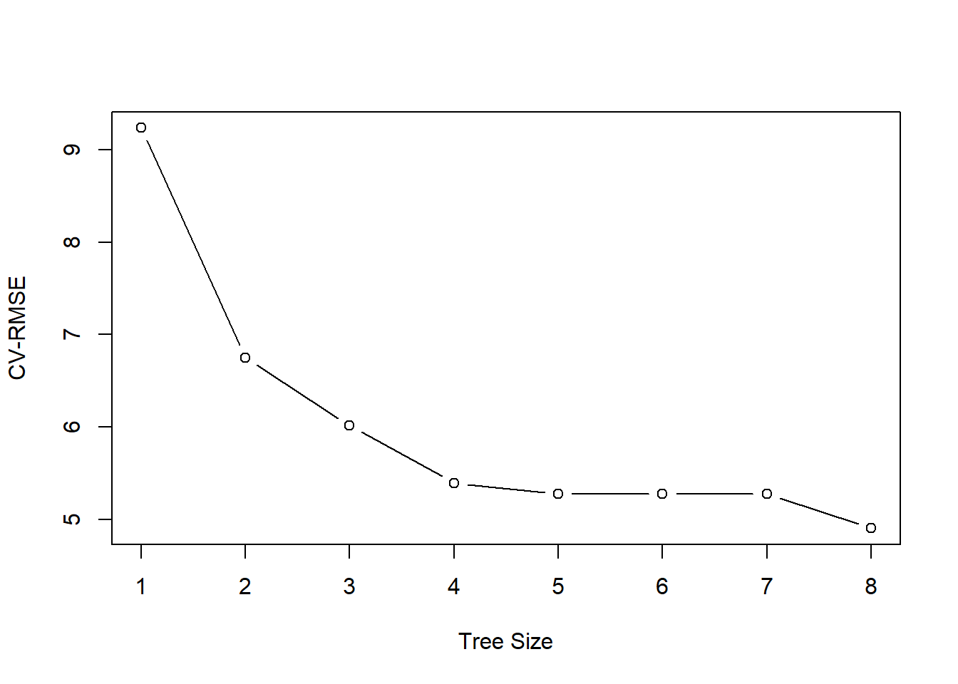
To do so, we’ll need to perform cross-validation and select the best subtree based on the RMSE score. This is achieveable with the cv.tree() function from the tree library.
# Perform CVset.seed(310)tree_cv =cv.tree(atree,K=10) # For more detail, type: ?cv.tree()plot(tree_cv$size, sqrt(tree_cv$dev /nrow(train)), type ="b",xlab ="Tree Size", ylab ="CV-RMSE")
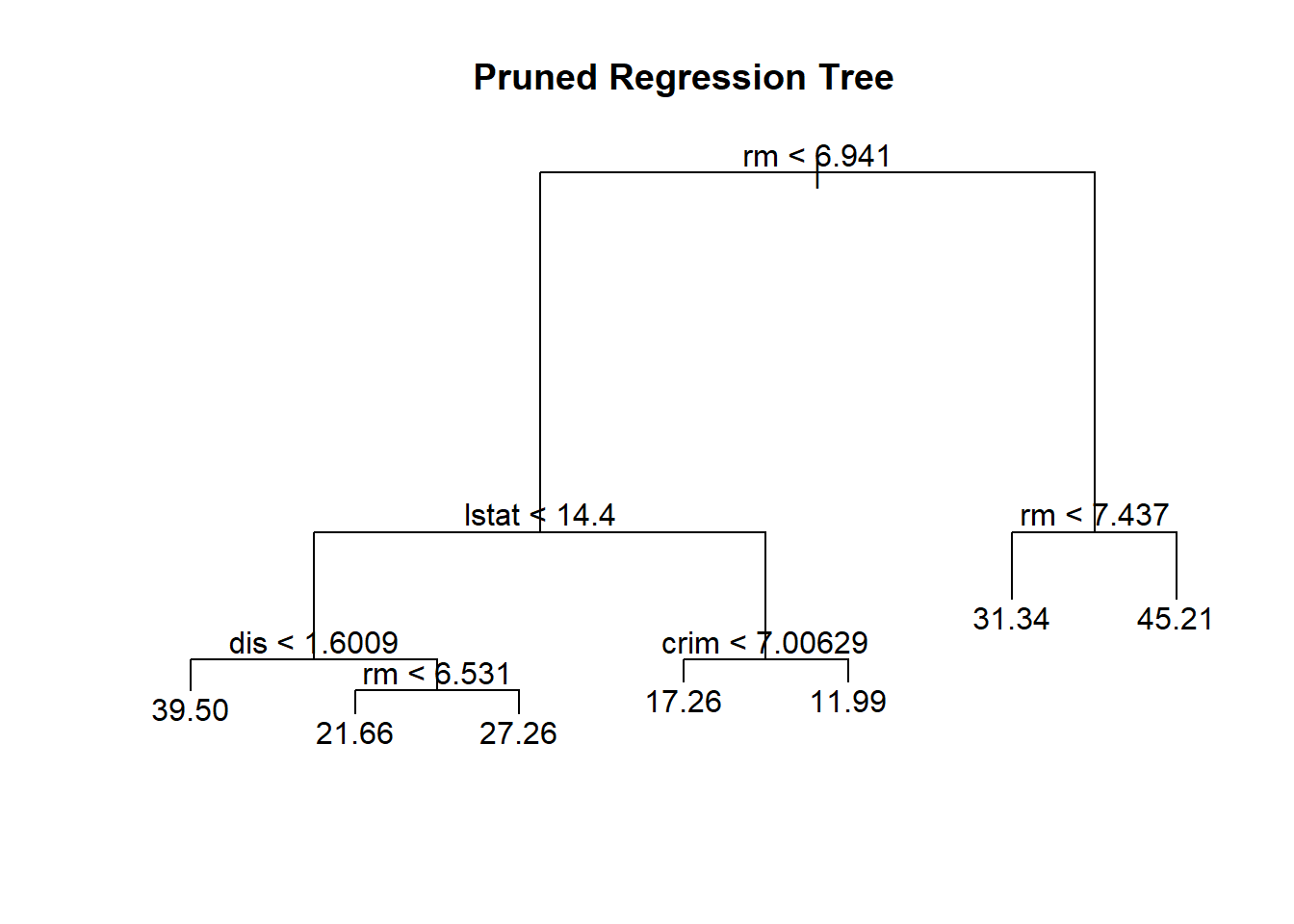
While the tree of size 8 does have the lowest RMSE, we’ll prune to a size of 7, since from 7 to 8, the difference is not as dramatic and it seems to perform just as well (otherwise, we would not be pruning).
We’ll take a look at the pruned tree below:
tree_prune =prune.tree(atree, best =7)summary(tree_prune)
Regression tree:
snip.tree(tree = atree, nodes = 6L)
Variables actually used in tree construction:
[1] "rm"    "lstat" "dis"   "crim"
Number of terminal nodes:  7
Residual mean deviance:  16.82 = 6677 / 397
Distribution of residuals:
    Min.  1st Qu.   Median     Mean  3rd Qu.     Max.
-23.3100  -2.0740   0.2146   0.0000   2.2380  14.5400
As expected, the pruned tree is smaller and easier to interpret compared to the unpruned tree, although the changes aren’t drastic. Now let’s take a look at the RMSE scores on the training and testing datasets:
tree.pred.train =predict(tree_prune, newdata = train)tree.pred.test =predict(tree_prune, newdata = test)# find RMSE on training and testingtree.rmse.trt =myRMSE(train$medv,tree.pred.train)tree.rmse.tst =myRMSE(test$medv,tree.pred.test) c( tree.rmse.trt, tree.rmse.tst )
[1] 4.065300 5.190901
Model Type
RMSE Score (Training)
RMSE Score (Testing)
Unpruned Tree
4.52
5.53
Pruned Tree
4.07
5.19
The lower RMSE scores show that the pruned tree performs considerably better than the unpruned tree as well.
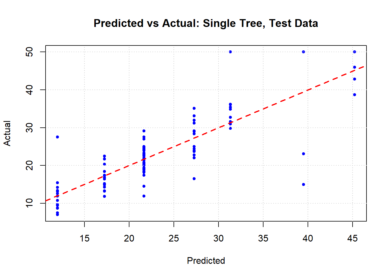
plot(tree.pred.test, test$medv, xlab ="Predicted", ylab ="Actual", main ="Predicted vs Actual: Single Tree, Test Data",col ="blue", pch =20)grid()abline(0, 1, col ="red", lty=2,lwd =2)
Creating a linear regression model for comparison
Since regression trees and linear regression models both work on the same type of continuous, numerical data, we’ll create a linear regression model, denoted mod.lin, and run it on the same testing and training data.
mod.lin =lm(medv~.,data=train)pred.train =predict(mod.lin, newdata=train)pred.test =predict(mod.lin,newdata=test)# Find RMSE on training and testinglin.rmse.trt =myRMSE(train$medv,pred.train)lin.rmse.tst =myRMSE(test$medv,pred.test)c( lin.rmse.trt, lin.rmse.tst)
[1] 4.596217 5.463523
Model Type
RMSE Score (Training)
RMSE Score (Testing)
Unpruned Tree
4.52
5.53
Pruned Tree
4.07
5.19
Linear Regression
4.60
5.46
The performance on the testing data indicates that linear regression performs at par, or slightly better than the unpruned tree on the Boston dataset, although it falls short of the pruned tree performance.
The rpart Package
The rpart package provides an alternative method for for fitting trees in R. It’s much more feature rich, including multiple cost complexity fits and performs cross-validation by default. It also has the ability to produce much nicer-looking trees. Based on its default settings, it will often result in smaller trees compared to using the tree package.
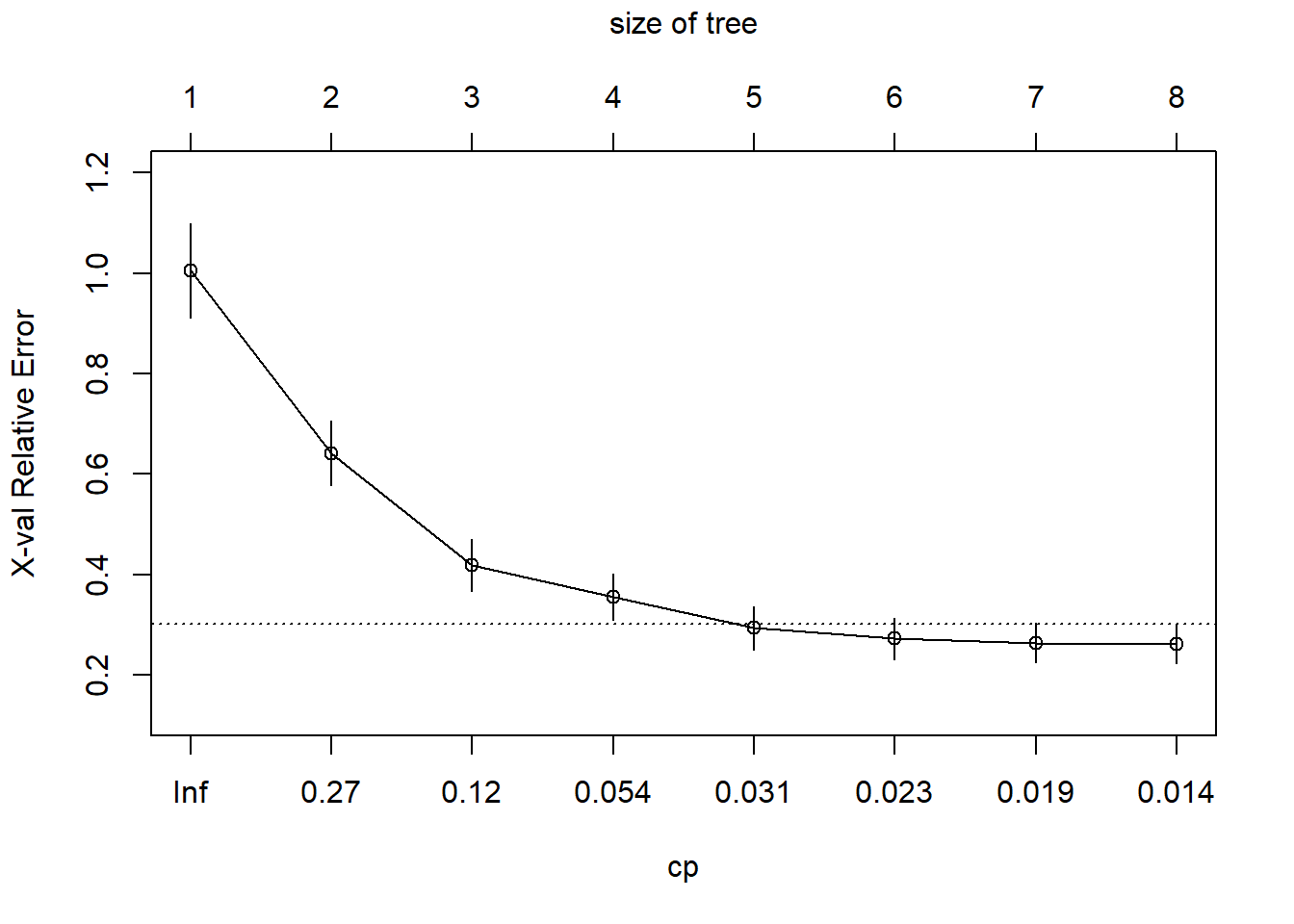
# install.packages("rpart")library(rpart)set.seed(310)medv.rpart =rpart(medv~., data=train)# Plot the cv error curve for the tree# rpart tries different cost-complexities by default# Also stores cv resultsplotcp(medv.rpart)
Pruning in rpart
rpart also comes with a prune() function, which takes a rpart-generated tree and a minimum cost-complexity value:
# Find the best cost-complexity valuemin_cp = medv.rpart$cptable[which.min(medv.rpart$cptable[,"xerror"]),"CP"]min_cp
[1] 0.01
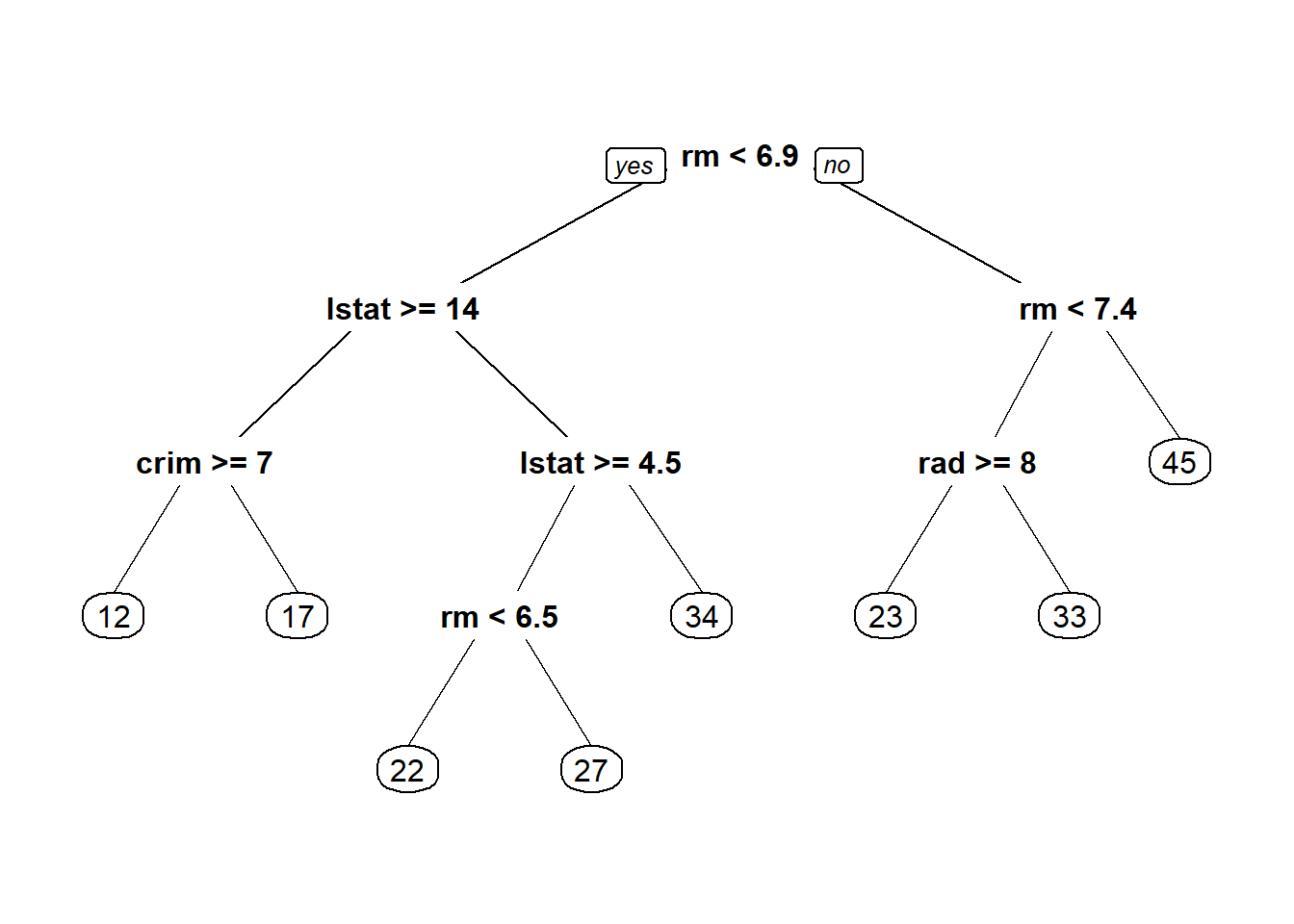
# Prune tree using best cost-complexityrpart.prune =prune(medv.rpart, cp = min_cp)
Plots in rpart
The rpart.plot library comes with a plot function that automatically generates nicer-looking tree graphs without overlap by calling the prp() function, which takes in a rpart-generated tree.
We’ll use the randomForest package to fit a bagged model. The act of bagging is actually a special case of a random forest where mtry (the number of variables to randomly sample as candidates in each split) is equal to p (total number of predictors). Usually, we only consider mtry out of full p predictors each time we decide on a tree split.
The opposite of a bagged model is a Random Forest model, where the variables used in each tree are randomly selected. Bagged models will use all of the features in all trees.
Call:
 randomForest(formula = medv ~ ., data = train, mtry = 12, type = "regression",      importance = TRUE, ntrees = 500)
               Type of random forest: regression
                     Number of trees: 500
No. of variables tried at each split: 12

          Mean of squared residuals: 10.87439
                    % Var explained: 87.21
Note that in the Boston dataset, there are only 12 variables excluding medv, since medv is the variable we are predicting. Which means in this case, p would equal 12, and the mtry value here is also 12.
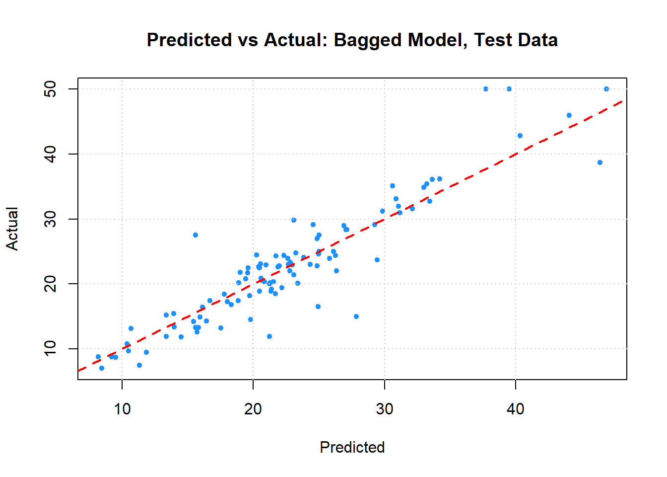
This is a large improvement over the previous models, however, the difference in the training and testing RMSE scores indicates that there may be a case of overfitting.
This may be due to the condition where bagging sometimes gives us trees that are highly correlated since the bagging method builds lots of similar trees. As such, averaging highly correlated values doesn’t reduce variance as much as averaging uncorrelated quantities.
# plot actual Y and predicted Y# if data points are close to the diagonal line, it means good predictionplot(bag.pred.test,test$medv,xlab ="Predicted", ylab ="Actual",main ="Predicted vs Actual: Bagged Model, Test Data",col ="dodgerblue", pch =20)grid()abline(0, 1, col ="red", lty=2,lwd =2)
Random Forest model
Now, we’ll try a Random Forest model. When creating a Random Forest for regression, the general suggestion is to try: mtry = sqrt(p), which would be rounded to 4, in this case.
For this, we’ll continue to use the randomForest() function from the randomForest package. The setup is similar to a bagged model.
Call:
 randomForest(formula = medv ~ ., data = train, mtry = 4, type = "regression",      importance = TRUE, ntrees = 500)
               Type of random forest: regression
                     Number of trees: 500
No. of variables tried at each split: 4

          Mean of squared residuals: 10.12727
                    % Var explained: 88.09
From the output above, you’ll see that we’ve generated this tree with similar parameters to the bagged model for comparison purposes. Both forests have 500 trees, as well as a similar percentage of variation explained.
To evaluate our Random Forest Model, we’ll go ahead and find the RMSE values on our testing and training datasets.
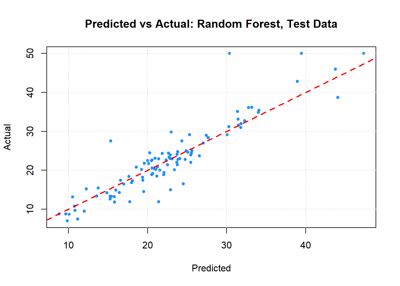
The RMSE scores are slightly worse than the bagged forest model, and also seems to have a discrepancy between the training and test scores. However, the trees generated in a Random Forest are generally less complex than a bagged model due to the random feature selection.
plot(forest.pred.test, test$medv,xlab ="Predicted", ylab ="Actual",main ="Predicted vs Actual: Random Forest, Test Data",col ="dodgerblue", pch =20)grid()abline(0, 1, col ="red", lty=2,lwd =2)
Ranking predictors
Since a Random Forest model doesn’t use all the predictors, we can find out which ones the model deems as most important using the importance() function from the randomForest package.
There are two ways to rank importance in predictors:
By the mean decrease in accuracy.
By the mean decrease in node impurity (Gini index score).
importance(forest, type =1) # List of predictors vs % change in MSE
%IncMSE
crim
15.4629939
zn
3.7184309
indus
11.9821826
chas
0.8484559
nox
17.3413671
rm
33.9691299
age
12.6821849
dis
19.0078660
rad
6.4064339
tax
12.4259294
ptratio
16.9473507
lstat
29.8890534
To further visualize this, we can plot out the difference in rankings using the function varImpPlot():
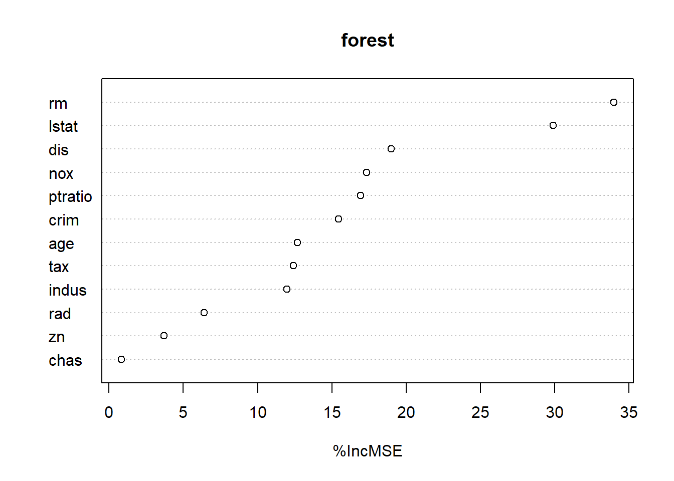
# Plot predictors in order of importance (most to less)varImpPlot(forest, type =1)
Here, it shows that the average number of rooms (rm) is by far the most important predictor for medv, however, the percentage of population considered lower status (lstat), is not too far behind.
Boosting
Lastly, we’ll try a boosted model, which by default will produce a nice predictor importance plot for us, as well as plots of the marginal effects of the predictors. For this, we’ll use the gbm package.
boost =gbm(medv ~ ., data = train, distribution ="gaussian", n.trees =5000, interaction.depth =4, shrinkage =0.1)boost
gbm(formula = medv ~ ., distribution = "gaussian", data = train,
    n.trees = 5000, interaction.depth = 4, shrinkage = 0.1)
A gradient boosted model with gaussian loss function.
5000 iterations were performed.
There were 12 predictors of which 12 had non-zero influence.
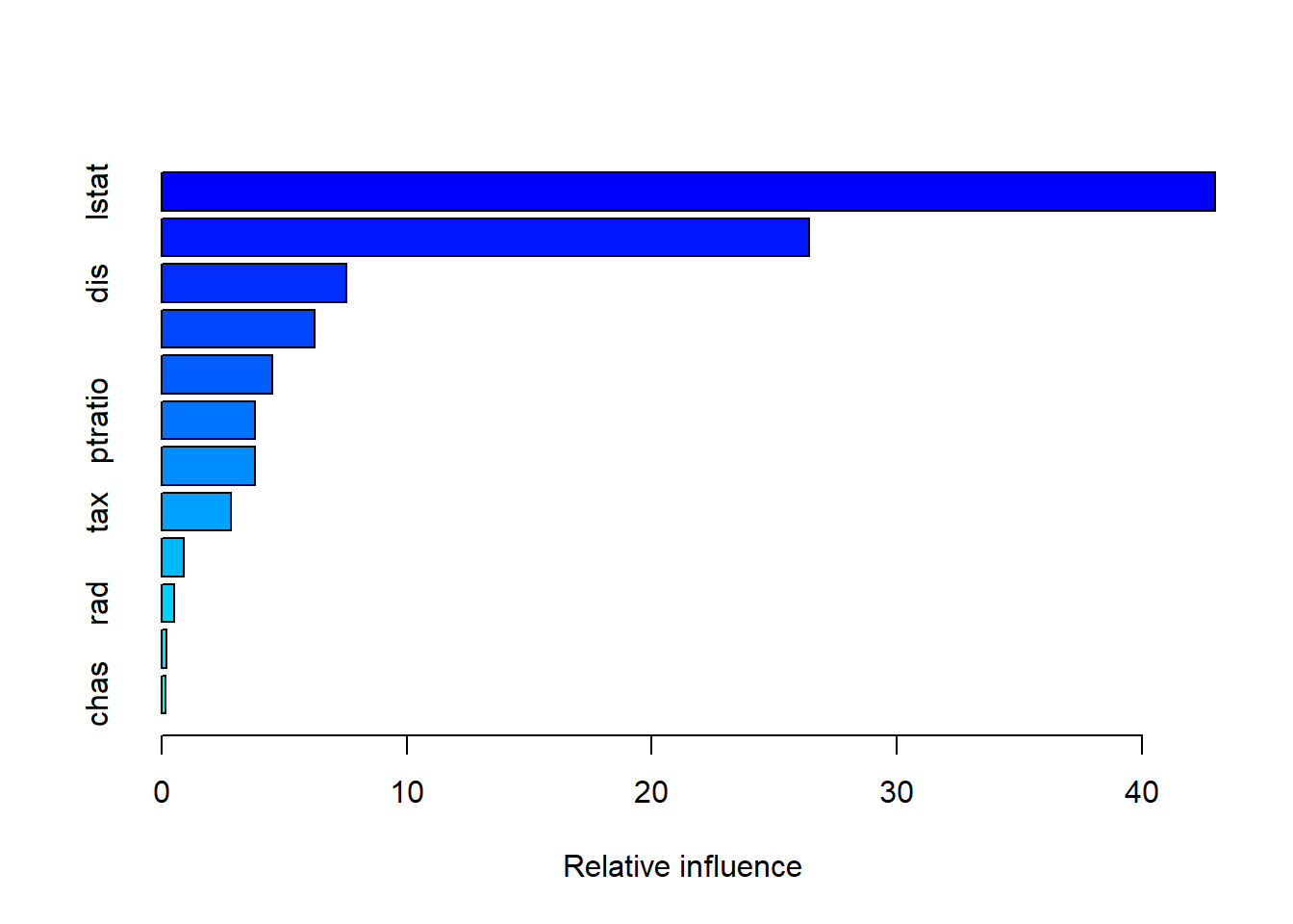
The output above states all 12 predictors have some level of influence over predicting the outcome variable (medv). Though, how much influence does each one have exactly? To visualize this, we’ll use the summary() function on our boosted tree model.
summary(boost)
var
rel.inf
lstat
lstat
42.9934534
rm
rm
26.4241420
dis
dis
7.5388505
crim
crim
6.2457069
age
age
4.5348747
ptratio
ptratio
3.8283260
nox
nox
3.8155045
tax
tax
2.8332332
indus
indus
0.8911894
rad
rad
0.5318406
zn
zn
0.1944506
chas
chas
0.1684282
Similarly, to varimplot(), lstat and rm remain the most influential predictors, however, their rankings are reversed this time with lstat much further ahead than rm.
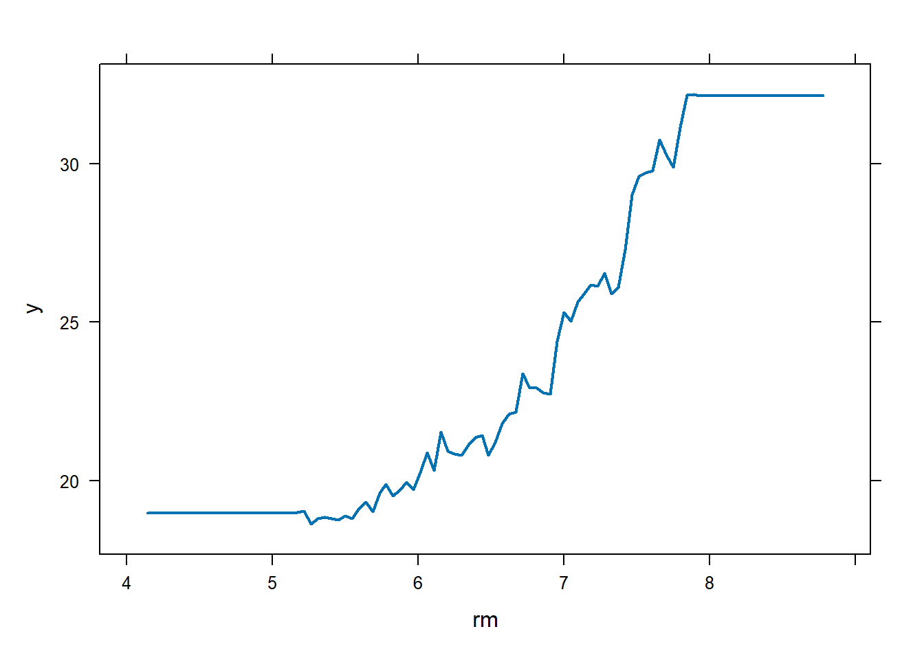
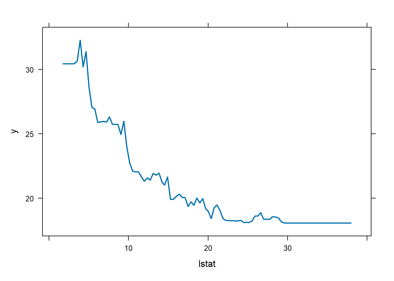
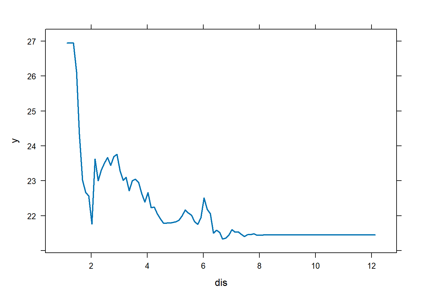
Below, we’ll plot the marginal effects of the three highest predictors:
plot(boost, i ="rm", col ="dodgerblue", lwd =2)plot(boost, i ="lstat", col ="dodgerblue", lwd =2)plot(boost, i ="dis", col ="dodgerblue", lwd =2)
Performance Summary
Now that all the models have been produced, we need to get the RMSE score of the boosted model before we can make the final summary:
For this data, tree-based methods outperform linear regression, among the tree methods, ensemble tree methods outperform single tree methods. The overall best method on this data is the bagging method with the lowest RMSE score (3.52) on the testing data set.
Why do ensemble models perform well? This is because ensemble methods such as Random Forests and boosting are ideal for reducing variance in models, which increase the accuracy of predictors.
Ensemble models reduce variance by training many trees on different data samples, and then averaging their predictions to come to a conclusion. An ensemble hinges on creating a diverse set of trees to mitigate biases that might exist in individual models.
The Random Forest method allows ensembles to introduce randomness into its trees by giving each tree a random subset of the data features.
The bagging method allows ensembles to introduce randomness into its trees by randomly subsetting the training data given to each tree.
Regression tree example with categorical predictors (Li, L. 2019. Towards Data Science.)Regression tree example with numerical predictors (Neufield, A. Treevalues.)