import numpy as np
import pandas as pd
import seaborn as sns
import matplotlib.pyplot as plt
import warnings
import os
warnings.filterwarnings('ignore')Neural Networks in Python
Outside of just R, there are several programming languages that provide powerful tools for statistical computation, and Python is one of them!
Python has libraries such as TensorFlow that provides support for creating complex machine-learning models, such as neural networks. Additionally, the language is known to be easy to read, making it a good entryway to statistical computing.
Due to Python’s expansive library and readability, it’s become an industry standard language in data science!
Jupyter Notebook for Python
Conveniently, Jupyter Notebook provides both R and Python support in its code cell format that was demonstrated in the Introductory Chapter, allowing us to run code in the Python language in a similar fashion to how we have been doing so with R.
Jupyter should come pre-installed with the IPython kernel, which means it should be ready for use from the get-go.
However, in the scenario that it is not, we’ll need to install the Python language first:
Installing language kernels in Jupyter
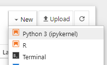
Once everything is correctly set up, you should have this option when choosing to create a new Jupyter notebook:
Python Packages
Numpy
Numpy is a package in Python that allows us to create vectors and index them similarly to how R functions. It also additionally supports operations created on those vectors, and is a keystone to data science in Python.
Pandas
Pandas is a data analysis and manipulation tool that works well with Numpy, having additional support for data structures such as dataframes
Seaborn
Seaborn is a data visualization tool that allows us to create graphs to accompany our data. It’s a visual library that requires matplotlib as the base plotting package.
Loading the Dataset
We’ll start by loading in both the training dataset and testing dataset used for our neural network.
# Training dataset
train = pd.read_csv("./mnist_train.csv")
#print(train.shape)
#train.head()

# Testing dataset
test= pd.read_csv("./mnist_test.csv")
#print(test.shape)
#test.head()
Data tidying
Additionally, we’ll want to clean the dataset for proper usage. We don’t want the ‘label’ column in here as it isn’t necessary for our model training.
We can do so using the drop method, where we specify the index to drop a row or column, as well as the axis.
When the
axis = 1, it tells Python that we are dropping a column.axis = 0indicates that a row is being dropped.
Y_train = train["label"]
X_train = train.drop(labels = ["label"],axis = 1)

Y_test = test["label"]
X_test = test.drop(labels = ["label"],axis = 1)
Dataset visualization
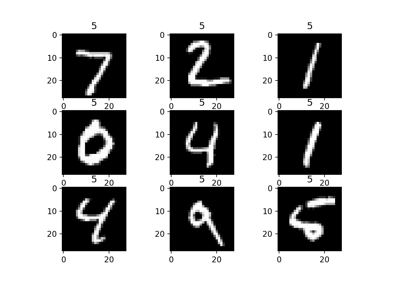
To demonstrate plotting functionality in Python, as well as the data distribution that we are working with here, we can plot the first 9 digits of the each dataset. Additionally, we’ll take a look at the data distribution of digit classes.
# Show distribution of digit classes
Y_train.value_counts()
label
1 6742
7 6265
3 6131
2 5958
9 5949
0 5923
6 5918
8 5851
4 5842
5 5421
Name: count, dtype: int64# Plot the first 9 digits in training set
for i in range(9):
img = X_train.iloc[i].to_numpy()
img = img.reshape((28,28))
plt.subplot(330+1+i) ## 33i: split the panel into 3X3, put plot on i position
plt.imshow(img,cmap='gray')
plt.title(train.iloc[0,0])
plt.show()
# Plot the first 9 digits in testing set
for i in range(9):
img = X_test.iloc[i].to_numpy()
img = img.reshape((28,28))
plt.subplot(330+1+i)
plt.imshow(img,cmap='gray')
plt.title(train.iloc[0,0])
plt.show()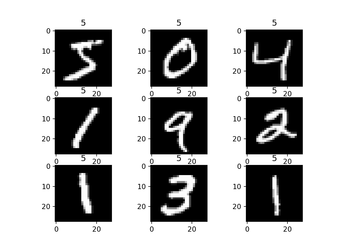
Normalization, Reshaping, and Label Encoding
As seen in Predictors and Transformers, we may want to refactor the data in ways that make it easier for the model to understand without the human context it has. Normalization and reshaping in Python allows us to perform these tasks.
# Normalize the data
X_train = X_train / 255.0
X_test = X_test / 255.0
print("x_train shape: ",X_train.shape)
print("x_test shape: ",X_test.shape)
x_train shape: (60000, 784)
x_test shape: (10000, 784)# Reshaping
X_train = X_train.values.reshape(-1,28,28,1)
X_test = X_test.values.reshape(-1,28,28,1)
print("X_train shape: ",X_train.shape)
print("X_test shape: ",X_test.shape)X_train shape: (60000, 28, 28, 1)
X_test shape: (10000, 28, 28, 1)Label encoding is a common technique used for converting categorical variables into numerical variables, where each unique category value is assigned a unique integer based on ordering (either alphabetical or numerical ordering).
We’ll be specifically using a label encoding technique called one-hot encoding, which allows us to represent the categorical variables as binary vectors.
# Label Encoding
from keras.utils import to_categorical # convert to one-hot-encoding
Y_train = to_categorical(Y_train, num_classes = 10)
Model training in Python
As we’ve done before, we’ll need to properly split the data for training. When doing so in Python, we have to separate the predictors (x-values) and the true category data (y-values).
from sklearn.model_selection import train_test_split
X_train, X_val, Y_train, Y_val = train_test_split(X_train, Y_train, test_size = 0.1, random_state=2)
print("X_train shape",X_train.shape)
print("X_val shape",X_val.shape)
print("Y_train shape",Y_train.shape)
print("Y_val shape",Y_val.shape)
X_train shape (54000, 28, 28, 1)
X_val shape (6000, 28, 28, 1)
Y_train shape (54000, 10)
Y_val shape (6000, 10)# Some examples
plt.imshow(X_train[1][:,:,0],cmap='gray')
plt.show()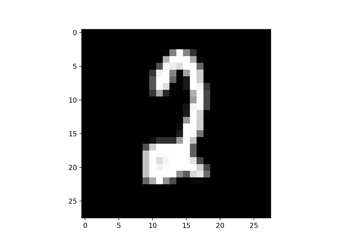
Convolutional Neural Network
A convolutional neural network (better known as CNN) is a type of network model that has layers specifically designed for image classification and object detection.
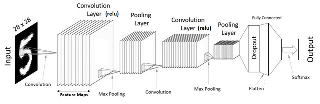
In total, CNN has three types of layers that are utilized:
Convolution layers
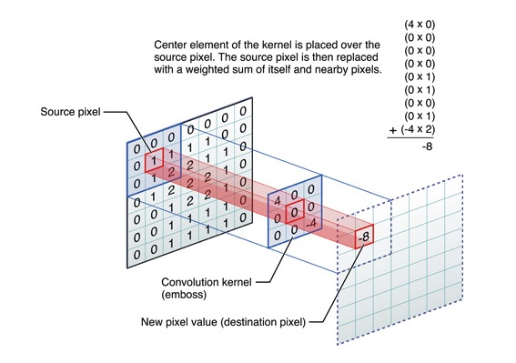
Convolutional layers are the foundation of CNN models – its main purpose is to extract features to distinguish images from one another. In short, it uses operators to convolute the input image, which simplifies the distinct features of each image and saves the convolution results.
Pooling layers
These layers are also known as ‘downsample layers’, as it reduces the dimensions of the feature maps (dataset features). It helps optimize the computing time of a CNN model by reducing the number of parameters to learn.
Additionally, the reduction in parameters may help the model from becoming too complex, reducing the risk of overfitting our data.
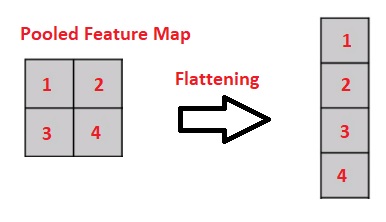
Flatten layers
At the end of a CNN model, we encapsulate the resulting data using a fully-connected (flatten) layer, which takes the high-level features extracted in the earlier layers to make predictions.
Creating a CNN Model
For our CNN, we’ll use a sequential model, which is a linear stack of layers. We’ll initialize it first, and then continue to add layers using the add method.
You could also add all layers at the initialized state.
from sklearn.metrics import confusion_matrix
import itertools

from keras.utils import to_categorical # convert to one-hot-encoding
from keras.models import Sequential
from keras.layers import Dense, Dropout, Flatten, Conv2D, MaxPool2D
from keras.optimizers import RMSprop,Adam
from keras.preprocessing.image import ImageDataGenerator
ImportError: cannot import name 'ImageDataGenerator' from 'keras.preprocessing.image' (C:\Users\joyli\AppData\Local\Programs\Python\PYTHON~1\Lib\site-packages\keras\api\preprocessing\image\__init__.py)from keras.callbacks import ReduceLROnPlateau
model = Sequential()Model layers in Python (Convolution + Pooling)
The layers we are adding will be as follows:
Conv2D, a 2-dimensional convolutional layer. The parameters used are:
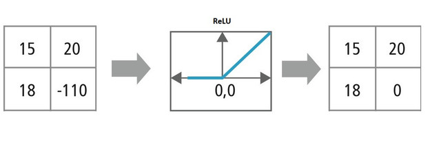
filters: the number of filters (kernels) used in the layerKernel_size: the dimension of the kernelpadding: there’s three relevant padding types in deep learning. We’ll keep the padding the same, which means our image size will be kept. (This is also called “zero padding” in deep-learning context).activation: the activation function used.input_shape: the shape of the image presented to the CNN model. In our case, our images are in a 28 x 28 dimension.
model.add(Conv2D(filters = 8, kernel_size = (5,5),padding = 'Same',
activation ='relu', input_shape = (28,28,1)))MaxPooling2D, a pooling operation for spatial data. The parameters used here are:
pool_size: in this case, our pool size is(2, 2), representing the factors to downscale in both directions.strides:(2, 2), the operation would then be moved down two rows, and back to the first column before continuing the process again.
model.add(MaxPool2D(pool_size=(2,2)))Dropout, a layer that randomly sets a fraction rate of input units to 0, which helps prevent overfitting. It uses one parameter, rate.
model.add(Dropout(0.25))Now, we’ll add the rest of the pooling and convolution layers, as a CNN model often has several of each before flattening the inputs.
model.add(Conv2D(filters = 16, kernel_size = (3,3),padding = 'Same',
                 activation ='relu'))
model.add(MaxPool2D(pool_size=(2,2), strides=(2,2)))
model.add(Dropout(0.25))
Flattening layer in Python
Once the other layers are set up, we can create our flattening layers.
flatten, a layer that flattens the input (does not affect batch size). It’s used without parameters.
Dense: This layer is a regular, fully-connected neural network layer. It can be used without parameters, or with.
units: a positive integer. Indicates the dimensionality of the output space (which is 256 in this case).activation: activation function. For the final layer, we usesoftmaxactivation, which is the standard for multiclass classification.
model.add(Flatten())
model.add(Dense(256, activation = "relu"))
model.add(Dropout(0.5))
model.add(Dense(10, activation = "softmax"))
Model compilation
When compiling our model, we want to specify the following parameters:
- Loss
- Optimizer
- Metrics
For the optimizer, we’ll use the adam optimizer to change the learning rate of our model.
# Adam optimizer: Change the learning rate
optimizer = Adam(learning_rate=0.001, beta_1=0.98, beta_2=0.99)
To compile the model, we’ll use a categorical crossentropy compilier, which is used for models that deal with multi-class data.
# Compile the model
model.compile(optimizer = optimizer , loss = "categorical_crossentropy", metrics=["accuracy"])

model.summary()
Model: "sequential"
┌─────────────────────────────────┬────────────────────────┬───────────────┐
│ Layer (type) │ Output Shape │ Param # │
├─────────────────────────────────┼────────────────────────┼───────────────┤
│ conv2d (Conv2D) │ (None, 28, 28, 8) │ 208 │
├─────────────────────────────────┼────────────────────────┼───────────────┤
│ max_pooling2d (MaxPooling2D) │ (None, 14, 14, 8) │ 0 │
├─────────────────────────────────┼────────────────────────┼───────────────┤
│ dropout (Dropout) │ (None, 14, 14, 8) │ 0 │
├─────────────────────────────────┼────────────────────────┼───────────────┤
│ conv2d_1 (Conv2D) │ (None, 14, 14, 16) │ 1,168 │
├─────────────────────────────────┼────────────────────────┼───────────────┤
│ max_pooling2d_1 (MaxPooling2D) │ (None, 7, 7, 16) │ 0 │
├─────────────────────────────────┼────────────────────────┼───────────────┤
│ dropout_1 (Dropout) │ (None, 7, 7, 16) │ 0 │
├─────────────────────────────────┼────────────────────────┼───────────────┤
│ flatten (Flatten) │ (None, 784) │ 0 │
├─────────────────────────────────┼────────────────────────┼───────────────┤
│ dense (Dense) │ (None, 256) │ 200,960 │
├─────────────────────────────────┼────────────────────────┼───────────────┤
│ dropout_2 (Dropout) │ (None, 256) │ 0 │
├─────────────────────────────────┼────────────────────────┼───────────────┤
│ dense_1 (Dense) │ (None, 10) │ 2,570 │
└─────────────────────────────────┴────────────────────────┴───────────────┘
Total params: 204,906 (800.41 KB)
Trainable params: 204,906 (800.41 KB)
Non-trainable params: 0 (0.00 B)