library(ISLR2)
data(Carseats)
Carseats$Sales = as.factor(ifelse(Carseats$Sales <= 8, "Low", "High"))
table(Carseats$Sales)/nrow(Carseats)Classification Trees
Classification trees are based on the decision tree model. When comparing it to regression trees, classification trees are used to predict categorical data, such as whether an email is spam or not, while regression trees predict numerical data, such as housing prices.
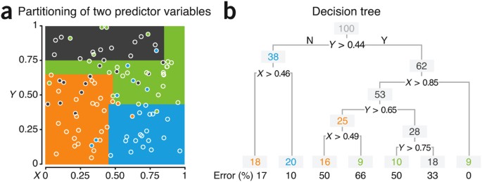
We’ll be working with concepts introduced in Regression Trees, such as pruning, random forest, and bagging.
One new concept introduced this chapter is boosting: an ensemble method where each new tree built works on improving the previously trained tree. This is different from Random Forest, and bagging, where each tree is independently trained, as boosted models only train one tree at a time.
The Carseat Dataset
To understand classification trees, we’ll use the Carseat dataset from the ISLR package. We’ll first modify the response variable Sales from its original use as a numerical variable, to a categorical variable with High for high sales, and Low for low sales.
Our process of building the models and comparing them will be similar to what was demonstrated in Regression Trees.
| Var1 | Freq |
|---|---|
| High | 0.41 |
| Low | 0.59 |
str(Carseats)'data.frame': 400 obs. of 11 variables:
$ Sales : Factor w/ 2 levels "High","Low": 1 1 1 2 2 1 2 1 2 2 ...
$ CompPrice : num 138 111 113 117 141 124 115 136 132 132 ...
$ Income : num 73 48 35 100 64 113 105 81 110 113 ...
$ Advertising: num 11 16 10 4 3 13 0 15 0 0 ...
$ Population : num 276 260 269 466 340 501 45 425 108 131 ...
$ Price : num 120 83 80 97 128 72 108 120 124 124 ...
$ ShelveLoc : Factor w/ 3 levels "Bad","Good","Medium": 1 2 3 3 1 1 3 2 3 3 ...
$ Age : num 42 65 59 55 38 78 71 67 76 76 ...
$ Education : num 17 10 12 14 13 16 15 10 10 17 ...
$ Urban : Factor w/ 2 levels "No","Yes": 2 2 2 2 2 1 2 2 1 1 ...
$ US : Factor w/ 2 levels "No","Yes": 2 2 2 2 1 2 1 2 1 2 ...Partitioning Data
Before we test and build our models, we need a proper training and testing set from Carseats. The process is the exact same as follows in Regression Trees.
set.seed(310)
index = sample(1:nrow(Carseats), nrow(Carseats)*0.8, replace=F)
train = Carseats[index,]
test = Carseats[-index,]

# Have a look of response distribution on train and test
table(train$Sales)/nrow(train)
table(test$Sales)/nrow(test)
   High     Low
0.40625 0.59375
 High   Low
0.425 0.575
The split between training and testing data has approximately a similar distribution, which is good for what we want to accomplish.
- For the training data, approximately 40.6% of entries are marked as high sales, and 59.4% are marked as low sales.
- For the testing data, approximately 42.5% of entries are marked as high sales, and 57.5% are marked as low sales.
Logistic Regression Model
Instead of linear regression, we’ll be using a logistic regression model and the glm() function due to the qualitative nature of our Y-value.
mod.glm = glm(Sales~., data=train, family=binomial)
# summary(mod.glm) for further details.

glm.pred.probtrn = predict(mod.glm, newdata=train, type="response")
glm.pred.probtst = predict(mod.glm, newdata=test, type="response")
cbind(train$Sales[1:5],glm.pred.probtrn[1:5])
[,1] [,2]
9 2 0.891240929
148 1 0.001348679
332 1 0.246067625
109 2 0.998544237
354 1 0.060251506We see that for the first five predictions, the logistic regression model uses 1 to indicate a high sales prediction, and 2 to indicate a low sales prediction.
For the overall predictions, we’ll use a confusion matrix as well as the accuracy test scores to benchmark our model.
glm.pred.train = ifelse(glm.pred.probtrn>=0.5, "Low","High")
table(train$Sales,glm.pred.train)

glm.pred.test = ifelse(glm.pred.probtst>=0.5, "Low","High")
table(test$Sales,glm.pred.test)

# Find accuracy rate on training set
glm.acc.trn = mean(glm.pred.train==train$Sales)
glm.acc.trn

# Find accuracy rate on testing set
glm.acc.tst = mean(glm.pred.test==test$Sales)
glm.acc.tst| High | Low | |
|---|---|---|
| High | 115 | 15 |
| Low | 13 | 177 |
| High | Low | |
|---|---|---|
| High | 30 | 4 |
| Low | 7 | 39 |
[1] 0.9125[1] 0.8625Unpruned Classification Tree
The rpart() and tree() function for creating classification trees uses the same parameters as a regression tree would, automatically adjusting its functions based on the input data.
library(rpart)
tree = tree(Sales ~ ., data = train)

summary(tree)
Classification tree:
tree(formula = Sales ~ ., data = train)
Variables actually used in tree construction:
[1] "ShelveLoc"   "Price"       "Advertising" "Income"      "CompPrice"
[6] "Population"  "Age"         "Education"
Number of terminal nodes:  27
Residual mean deviance:  0.3703 = 108.5 / 293
Misclassification error rate: 0.1 = 32 / 320
We see here that the tree has 27 terminal nodes, and a misclassification rate of 0.10 (10%).
We’ll plot it next to see how to visualize it:
plot(tree)
text(tree, pretty = 0)
title(main = "Unpruned Classification Tree")
Now to get the accuracy scores between the training and testing sets:
set.seed(12)

tree.pred.trt = predict(tree,train, type="class")
tree.acc.trn = mean(tree.pred.trt==train$Sales)
table(train$Sales,tree.pred.trt)

tree.pred.tst = predict(tree,test, type="class")
tree.acc.tst = mean(tree.pred.tst==test$Sales)
table(test$Sales,tree.pred.tst)

tree.acc.trn
tree.acc.tst| High | Low | |
|---|---|---|
| High | 122 | 8 |
| Low | 22 | 168 |
| High | Low | |
|---|---|---|
| High | 26 | 8 |
| Low | 10 | 36 |
[1] 0.90625[1] 0.775So far, with the unpruned classification tree, we have a training score of 0.91 and a testing score of 0.78, which is slightly worse than the logistic regression model but not too far behind.
| Model Type | Training Score | Testing Score |
|---|---|---|
| Logistic Regression | 0.91 | 0.86 |
| Unpruned Tree | 0.91 | 0.78 |
It’s easy to see that the tree has been overfit, since the training set performs much better than the test set.
Pruned Classification Tree
To attempt to improve the unpruned scores, we’ll use cross-validation to find trees of different sizes, which have been pruned from our original tree.
set.seed(3)
tree.cv = cv.tree(tree, FUN = prune.misclass)

plot(tree.cv$size, tree.cv$dev/nrow(train),
    type="b",
    xlab="Tree size",
    ylab = "CV mis-classification Rate")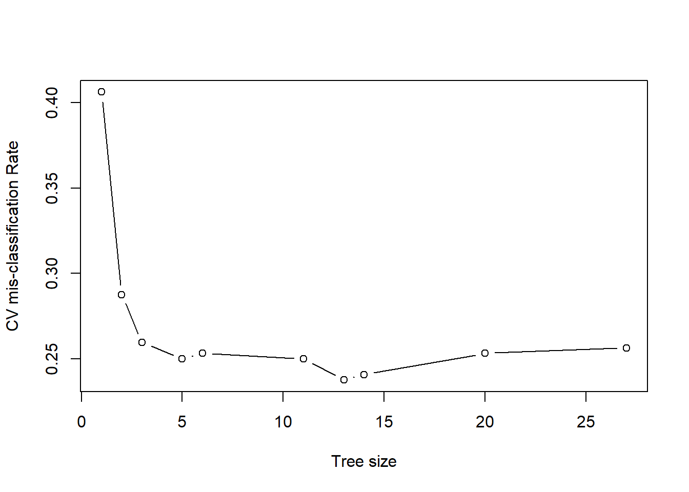
# Optimal tree size
tree.cv$size[tree.cv$dev/nrow(train)==min( tree.cv$dev/nrow(train) )]
[1] 13It appears that a tree of size 13 has the fewest misclassifications of all considered trees, shown via cross-validation. To obtain that size 13 tree, we’ll use prune.misclass().
tree.prune = prune.misclass(tree, best = 13)
summary(tree.prune)
Classification tree:
snip.tree(tree = tree, nodes = c(4L, 25L, 28L, 31L, 24L, 30L,
59L, 467L, 5L))
Variables actually used in tree construction:
[1] "ShelveLoc"   "Price"       "Advertising" "CompPrice"   "Age"
Number of terminal nodes:  13
Residual mean deviance:  0.6957 = 213.6 / 307
Misclassification error rate: 0.125 = 40 / 320 plot(tree.prune)
text(tree.prune, pretty = 0)
title(main = "Pruned Classification Tree")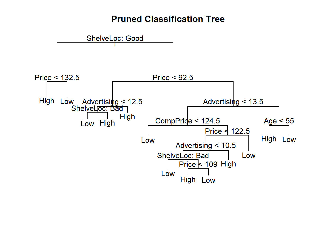
Now to get the accuracy scores between the training and testing sets:
set.seed(12)

tree.pred.trt = predict(tree.prune,train, type="class")
tree.acc.trn = mean(tree.pred.trt==train$Sales)
table(train$Sales,tree.pred.trt)

tree.pred.tst = predict(tree.prune,test, type="class")
tree.acc.tst = mean(tree.pred.tst==test$Sales)
table(test$Sales,tree.pred.tst)

tree.acc.trn
tree.acc.tst| High | Low | |
|---|---|---|
| High | 103 | 27 |
| Low | 13 | 177 |
| High | Low | |
|---|---|---|
| High | 20 | 14 |
| Low | 6 | 40 |
[1] 0.875[1] 0.75The training set performs almost as well as the unpruned one, however the difference between the test and training scores still shows overfitting. This is expected as trees tend to overfit. Continuing forward, we’ll look at several ways to fix this, including: bagging, boosting, and random forests.
| Model Type | Training Score | Testing Score |
|---|---|---|
| Logistic Regression | 0.91 | 0.86 |
| Unpruned Tree | 0.91 | 0.78 |
| Pruned Tree | 0.88 | 0.75 |
Bagged Forest
To start, we’ll load in the randomForest package to create a bagged model. The parameters and inputs are roughly the same as a regression model would be in randomForest(), except the type parameter would be "classification".
library(randomForest)

set.seed(310)
bag = randomForest(Sales ~ .,
                   data = train,
                   mtry = 10,
                   type="classification",
                   importance = TRUE,
                   ntrees = 500)
bag

varImpPlot(bag,type=2)
Call:
 randomForest(formula = Sales ~ ., data = train, mtry = 10, type = "classification",      importance = TRUE, ntrees = 500)
               Type of random forest: classification
                     Number of trees: 500
No. of variables tried at each split: 10

        OOB estimate of  error rate: 19.06%
Confusion matrix:
     High Low class.error
High   94  36   0.2769231
Low    25 165   0.1315789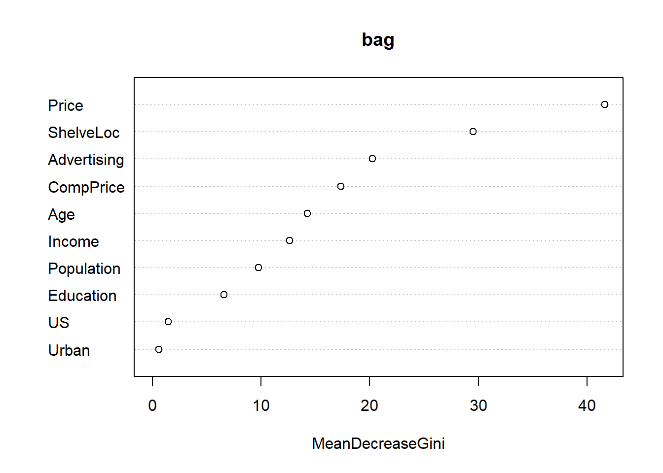
Here, we see that Price and ShelveLoc (shelf location) are the most influential predictors for Sales, with Advertising coming in third, according to the bagged model.
We’ll continue and calculate the scores:
bag.acc.trn = mean(train$Sales==predict(bag,newdata=train))
table(train$Sales,predict(bag,newdata=train))

bag.pred.tst = predict(bag,newdata=test)
table(test$Sale,bag.pred.tst)

bag.acc.trn
bag.acc.tst| High | Low | |
|---|---|---|
| High | 130 | 0 |
| Low | 0 | 190 |
| High | Low | |
|---|---|---|
| High | 24 | 10 |
| Low | 5 | 41 |
[1] 1[1] 0.825So far, the bagged model does a good job at improving the scores overall, compared to the other models. It has the highest training score, but also the largest gap between training and testing scores indicating this model is more overfit than the previous two.
| Model Type | Training Score | Testing Score |
|---|---|---|
| Logistic Regression | 0.91 | 0.86 |
| Unpruned Tree | 0.91 | 0.78 |
| Pruned Tree | 0.88 | 0.75 |
| Bagged Forest | 1.00 | 0.83 |
Random Forest
For Random Forest classifiers, the suggested mtry is similar to the Random Forest regressors, where mtry = sqrt(p).
\sqrt{p} = \sqrt{10} = 3 (We’ll round down.)
set.seed(10)
rdf = randomForest(Sales ~ .,
                   data = train,
                   mtry = 3,
                   type="classification",
                   importance = TRUE,
                   ntrees = 500)
rdf
Call:
 randomForest(formula = Sales ~ ., data = train, mtry = 3, type = "classification",      importance = TRUE, ntrees = 500)
               Type of random forest: classification
                     Number of trees: 500
No. of variables tried at each split: 3

        OOB estimate of  error rate: 18.75%
Confusion matrix:
     High Low class.error
High   91  39   0.3000000
Low 21 169 0.1105263varImpPlot(rdf)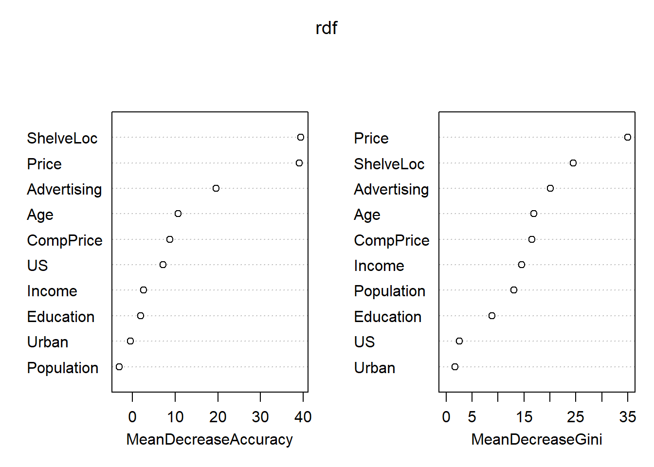
In the output above, ShelveLoc, Price, and Advertising are listed to be the most important predictors, similar to the bagged forest model, however, the individual rankings vary.
- Mean Decrease Accuracy: how much the model accuracy decreases if we drop that variable.
- Mean Decrease Gini: measure of variable importance based on the Gini impurity index used for the calculation of splits in trees.
Now, we’ll examine the accuracy scores on the training and testing sets:
rdf.acc.trn = mean(train$Sales==predict(rdf,newdata=train))
table(train$Sales,predict(rdf,newdata=train))
rdf.acc.tst = mean(test$Sales==rdf.pred.tst)

rdf.pred.tst = predict(rdf,newdata=test)
table(test$Sale,rdf.pred.tst)

rdf.acc.trn
rdf.acc.tst| High | Low | |
|---|---|---|
| High | 130 | 0 |
| Low | 0 | 190 |
| High | Low | |
|---|---|---|
| High | 23 | 11 |
| Low | 5 | 41 |
[1] 1[1] 0.8Overall, the performance of the Random Forest model is slightly below the bagged model. Though it’s possible with more experimentation and parameter alteration, the score could be further improved.
| Model Type | Training Score | Testing Score |
|---|---|---|
| Logistic Regression | 0.91 | 0.86 |
| Unpruned Tree | 0.91 | 0.78 |
| Pruned Tree | 0.88 | 0.75 |
| Bagged Forest | 1.00 | 0.83 |
| Random Forest | 1.00 | 0.80 |
Boosted Forest
To perform boosting, we’ll modify the response variable (Sales) to be 0 (High) and 1 (Low) to work with gbm. Later on, we’ll learn to use caret to fit gbm models, which will avoid this extra step.
There is one difference in parameters when building a classification model instead of a regression model with gbm, namely, that distribution = "bernoulli".
library(gbm)

seat.trn = train
seat.trn$Sales= ifelse(seat.trn$Sales=="Low",0,1)

boost = gbm(Sales ~ .,
            data = seat.trn,
            distribution = "bernoulli",
            n.trees = 5000,
            interaction.depth = 4,
            shrinkage = 0.01)
boost
gbm(formula = Sales ~ ., distribution = "bernoulli", data = seat.trn,
n.trees = 5000, interaction.depth = 4, shrinkage = 0.01)
A gradient boosted model with bernoulli loss function.
5000 iterations were performed.
There were 10 predictors of which 10 had non-zero influence.The above results show us that there are a total of 5000 trees generated, and that all of the predictors have a non-insignificant impact on the accuracy rate of the boosted model.
Performance Summary
Now that all the models have been produced, we need to get the last scores of the boosted model before we can make the performance summary:
# Acccuracy on train set
boost.pred.trn = ifelse(predict(boost, train, n.trees = 5000, "response") > 0.5,
                        "High", "Low")
table(train$Sales,boost.pred.trn)
boost.acc.trn = mean(train$Sales==boost.pred.trn)

# Accuracy on test set
boost.pred.tst = ifelse(predict(boost, test, n.trees = 5000, "response") > 0.5,
                        "High", "Low")
table(test$Sales,boost.pred.tst)
boost.acc.tst = mean(test$Sales==boost.pred.tst)

boost.acc.trn
boost.acc.tst
boost.pred.trn
High Low
High 130 0
Low 0 190 boost.pred.tst
High Low
High 28 6
Low 4 42[1] 1[1] 0.875| Model Type | Training Score | Testing Score |
|---|---|---|
| Logistic Regression | 0.91 | 0.86 |
| Unpruned Tree | 0.91 | 0.78 |
| Pruned Tree | 0.88 | 0.75 |
| Bagged Forest | 1.00 | 0.83 |
| Random Forest | 1.00 | 0.80 |
| Boosted Forest | 1.00 | 0.88 |
From the results, you could see most tree methods including ensemble methods are over fitting, but the logistic regression model achieves a good trade-off between overfitting and higher scores, meaning that it’s a better model for the data that we have.