library(MASS)
data(iris)
# First check that no datapoint is missing
apply(iris, 2, function(x) sum(is.na(x)))Neural Networks in R
A neural network is a machine-learning algorithm that makes decisions in a manner similar to our human brains. It uses interconnected nodes (neurons) in a layered structure and has an adaptive system that computers also use, which learn from their mistakes and improve continuously.
Neural networks can handle complicated problems such as summarizing documents, or recognizing faces, with generally greater accuracy than more other algorithms.

Packages
In this chapter, we’ll learn how to create neural networks in R, utilizing the neuralnet package!
We’ll use the iris dataset for our examples. The details of it can be found in the iris dataset overview. First, we’ll want to make sure our data is ready for model fitting.
| apply(iris, 2, function(x) sum(is.na(x))) | |
|---|---|
| Sepal.Length | 0 |
| Sepal.Width | 0 |
| Petal.Length | 0 |
| Petal.Width | 0 |
| Species | 0 |
The results for all of the categories returns as zero, which means there’s no missing data. Let’s proceed by randomly splitting the data into training and testing sets, which we’ll fit a linear regression and MLP model on.
Data Partitioning
The sample(x, size) function outputs a vector of the specified size from randomly selected samples in vector x. By default, the sampling is without replacement: the selected index is essentially a random vector of indeces.
- iris[index, ]: extract all rows from the full dataset with the selected row indices.
- iris[-index,]: extract all the rows from the full dataset that were not the selected row indices.
# data spliting
set.seed(310)
index = sample(1:nrow(iris), round(0.7*nrow(iris)), replace=F)
train = iris[index,]
test = iris[-index,]
dim(train)
[1] 105 5dim(test)[1] 45 5Training Models using neuralnet
To build neural network models in R, we’ll need to use the neuralnet package. The neuralnet(formula, data, hidden, linear.output) function has these following parameters we’ll use:
- formula:
y ~ predictors, the formula follows the same format as most other modelling functions in R. - data: a dataframe containing the variables listed in
formula. - hidden: a vector of integers specifying the number of hidden neurons in each layer.
- linear.output: by default, this is set to
FALSE. We’ll keep it this way.
# install.packages("neuralnet")
library(neuralnet)
nnet = neuralnet(Species~., train, hidden = c(4,3), linear.output = FALSE)
plot(nnet,rep="best")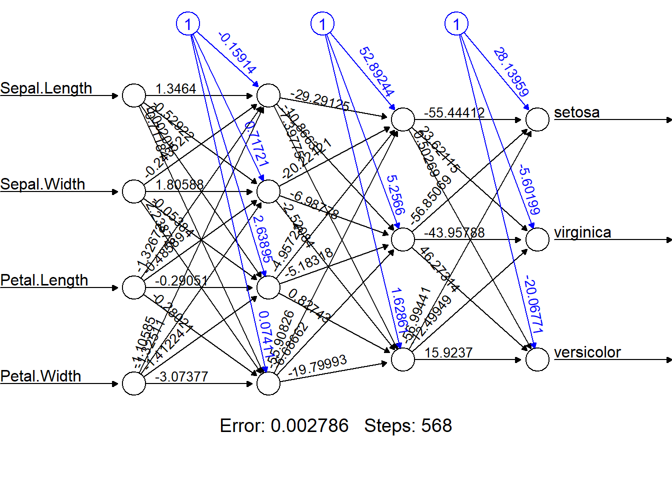
To obtain the outputs from running nnet on our test data, we’ll need to use the compute() function provided by neuralnet. (Note that you may need to write it was neuralnet::compute() to let R know that we’re overriding any native compute() functions.)
ypred = neuralnet::compute(nnet, test[,-5])
yhat = ypred$net.result
head(yhat)
[,1] [,2] [,3]
1 1 0.003676943 1.926207e-09
6 1 0.003676943 1.926207e-09
7 1 0.003676943 1.926207e-09
11 1 0.003676943 1.926207e-09
17 1 0.003676943 1.926207e-09
22 1 0.003676943 1.926207e-09The prediction results above show the probability of each class. We’ll have to extract the class with the highest probability values, as our final predicted result:
c("setosa","versicolor","virginica")[yhat[1,]==max(yhat[1,])]
sp = c("setosa","versicolor","virginica")
tt = apply(yhat,1,function(x) sp[x==max(x)])
tt
[1] "setosa"| tt | |
|---|---|
| 1 | setosa |
| 6 | setosa |
| 7 | setosa |
| 11 | setosa |
| 17 | setosa |
| 22 | setosa |
| 24 | setosa |
| 27 | setosa |
| 32 | setosa |
| 33 | setosa |
| 35 | setosa |
| 38 | setosa |
| 47 | setosa |
| 48 | setosa |
| 52 | versicolor |
| 53 | versicolor |
| 59 | versicolor |
| 61 | versicolor |
| 63 | versicolor |
| 64 | versicolor |
| 69 | versicolor |
| 71 | virginica |
| 74 | versicolor |
| 75 | versicolor |
| 79 | versicolor |
| 80 | versicolor |
| 82 | versicolor |
| 84 | virginica |
| 87 | versicolor |
| 89 | versicolor |
| 90 | versicolor |
| 97 | versicolor |
| 106 | virginica |
| 108 | virginica |
| 115 | virginica |
| 117 | virginica |
| 118 | virginica |
| 120 | virginica |
| 124 | virginica |
| 125 | virginica |
| 127 | virginica |
| 128 | virginica |
| 136 | virginica |
| 139 | virginica |
| 146 | virginica |
This outputs the prediction for each observation in the testing set. The index numbers on the left are the indices of each observation in the full Iris dataset, and the tt value is the final prediction for each observation.
Accuracy scores
We can view the accuracy of our neural network model by generating a confusion matrix:
yclass = apply(yhat,1,function(x) sp[x==max(x)])
# Same as: yclass= sp[ apply(yhat, 1, which.max) ]
table(test$Species, yclass)| setosa | versicolor | virginica | |
|---|---|---|---|
| setosa | 14 | 0 | 0 |
| versicolor | 0 | 16 | 2 |
| virginica | 0 | 0 | 13 |
print("Accuracy on testing dataset:")
mean(test$Species==yclass)
[1] "Accuracy on testing dataset:"[1] 0.9555556For a first attempt, a 95.6% accuracy rate is quite good compared to what we’ve gotten in the past with different models. Recall that our K-means model had an accuracy rate of 89% on its first attempt with the Iris dataset.
Training a second MLP model
Let’s explore what else neuralnet() has to offer, by starting with some more parameters:
- rep: the number of repetitions used for the neural network’s training.
- err.fct: a differentiable function that is used for the calculation of the error. Alternatively, the strings
"sse"and"ce"which stand for the sum of squared errors and the cross-entropy can be used. - lifesign: a string specifying hwo much the function will print during the calculation of the neural network. (
none,minimal, orfull.) - stepmax: the maximum steps for the training of the neural network. Reaching this maximum leads to a hard stop of the neural network’s training process.
- threshold: a numeric value specifying the theshold for the partial derivatives of the error function as a stopping criteria.
# Let's train another MLP model
iris.net <- neuralnet(Species ~ Sepal.Length + Sepal.Width + Petal.Length + Petal.Width,
                      data=train,
                      hidden=c(5,6),
                      rep = 3,
                      err.fct = "ce",
                      linear.output = F,
                      lifesign = "minimal",
                      stepmax = 1000000,
                      threshold = 0.001)
hidden: 5, 6 thresh: 0.001 rep: 1/3 steps: 3035 error: 5e-05 time: 0.7 secs
hidden: 5, 6 thresh: 0.001 rep: 2/3 steps: 1108 error: 3e-05 time: 0.17 secs
hidden: 5, 6 thresh: 0.001 rep: 3/3 steps: 808 error: 1e-04 time: 0.14 secsplot(iris.net, rep = 'best')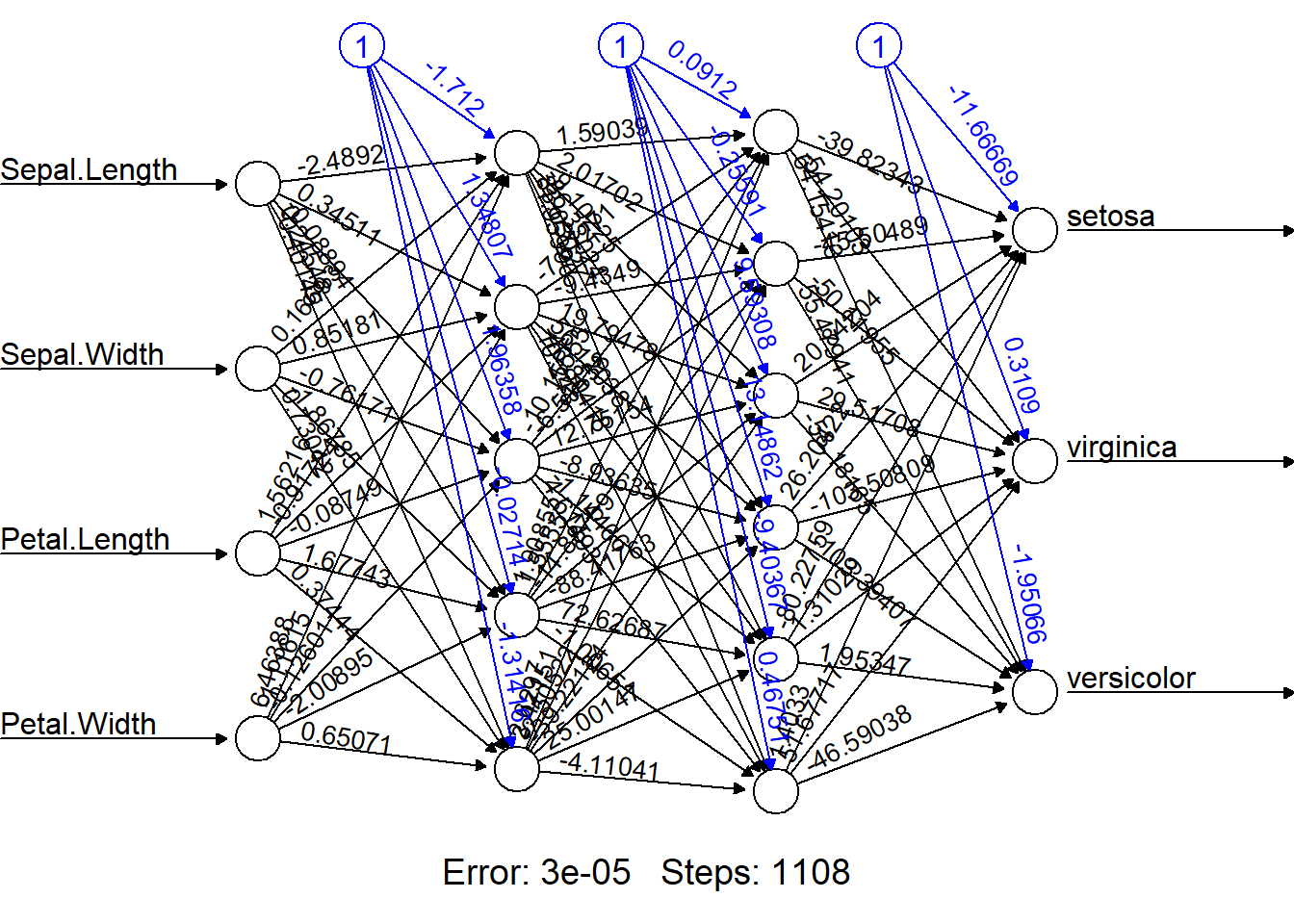
Let’s see what accuracy score our second neural network model has:
iris.pred = compute(iris.net, test[-5:-8])
idx = apply(iris.pred$net.result, 1, which.max)
preds = c('setosa', 'versicolor', 'virginica')[idx]
table(preds, test$Species)| setosa | versicolor | virginica | |
|---|---|---|---|
| setosa | 14 | 0 | 0 |
| versicolor | 0 | 16 | 0 |
| virginica | 0 | 2 | 13 |
print("Accuracy on the testing data set:")
mean(preds==test$Species)
[1] "Accuracy on the testing data set:"[1] 0.9555556