Multiple Linear Regression

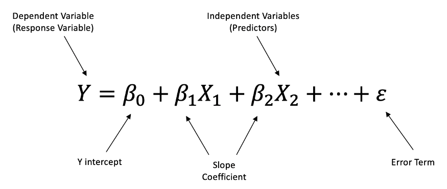
While simple linear regression uses one independent variable to predict the outcome of a dependent variable, multiple linear regression utilizes two or more independent variables. The flexibility of multiple linear regression allows us to capture the complex nature of real-world data, allowing us to account for more variables.

Generating a Multiple Linear Regression Fit

In order to fit a multiple linear regression model with least-squares, we’ll use the lm() function.

The lm() equation parameter can account for multiple variables, for example, the syntax lm(y ~ x1 + x2 + x3) fits a model with three predictors, x1, x2, and x3.

The summary() function now outputs the regression coefficients for all the predictors.

lm.fit <- lm(medv ~ lstat + age, data = Boston)
summary(lm.fit)


Call:
lm(formula = medv ~ lstat + age, data = Boston)

Residuals:
    Min      1Q  Median      3Q     Max 
-15.981  -3.978  -1.283   1.968  23.158 

Coefficients:
            Estimate Std. Error t value Pr(>|t|)    
(Intercept) 33.22276    0.73085  45.458  < 2e-16 ***
lstat       -1.03207    0.04819 -21.416  < 2e-16 ***
age          0.03454    0.01223   2.826  0.00491 ** 
---
Signif. codes:  0 '***' 0.001 '**' 0.01 '*' 0.05 '.' 0.1 ' ' 1

Residual standard error: 6.173 on 503 degrees of freedom
Multiple R-squared:  0.5513,    Adjusted R-squared:  0.5495 
F-statistic:   309 on 2 and 503 DF,  p-value: < 2.2e-16

The entire Boston dataset includes 12 variables, and if we wanted to use all of them as predictors for medv, it would be cumbersome to type all of these in the regression function. As an alternative, the short-hand to use all variables would be a period:

# Use all variables except medv as predictors for medv
lm.fit <- lm(medv ~ ., data = Boston) 
summary(lm.fit)

What if we wanted to perform a regression using all the variables available but one? For example, in the above regression output, age has a high p-value. So we may wish to run a regression excluding this predictor. The following syntax results in a regression using all predictors except age:

lm.fit1 <- lm(medv ~ . - age, data = Boston)
summary(lm.fit1)

Alternatively, the update() function provides the same results.

lm.fit1 <- update(lmfit, ~ . - age)

Accessing individual components of a summary

We can access the individual components of a summary object by name:

summary(lm.fit)$r.sq gives us R^2, the coefficient of determination.
summary(lm.fit)$sigma gives us RSE, the residual/relative standard error.

# Retrieving the correlation of determination value
summary(lm.fit)$r.sq

[1] 0.734307

# Retrieving the standard deviation value
summary(lm.fit)$sigma

[1] 4.798034

To explore addition functionality, type ?summary.lm in the Jupyter or R console to see what is available.

Variance Inflation Factor

The variance inflation factor (VIF) is important in multiple linear regression as it allows us to measure the amount of multicollinearity in regression analysis.

Multicollinearity is a statistical term that describes when two or more independent variables in a regression model are highly correlated. This indicates a strong linear relationship between the predictor variables.

Multicollinearity can be an issue, because when independent variables are highly correlated with one another, it can undermine the statistical significance of an independent variable. Generally, a VIF score above four indicates that multicollinearity might exist.

Computing VIF

The vif() function (part of the car package), computes variance inflation factors given a fitted model. In the Boston dataset, most VIF scores indicate a low or moderate correlation between predictors.

The car package is not part of the base R installation, so it must be downloaded the first time you use it via the install.packages() function, which is demonstrated in our library guide.

library(car)

vif(lm.fit)

    crim       zn    indus     chas      nox       rm      age      dis 
1.767486 2.298459 3.987181 1.071168 4.369093 1.912532 3.088232 3.954037 
     rad      tax  ptratio    lstat 
7.445301 9.002158 1.797060 2.870777

Judging from the output, our current lm.fit model has two independent variables that are much higher than the others: rad and tax.

Interaction Terms

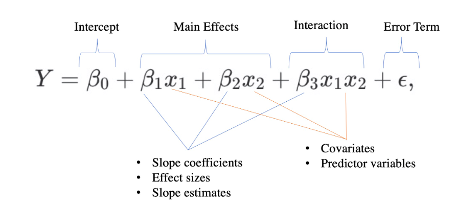
Interaction terms in multiple linear regression allows us to check whether the relationship between the dependent and independent variable changes depending on the value of another independent variable.

Regression model with an interaction term

Including interaction terms is easily done through lm().

The syntax var1:var2 tells R to include an interaction term between var1 and var2.
The syntax var1 * var2 will simultaneously include var1, var2, and the interaction term var1:var2 as predictors; it’s a shorthand for var1 + var2 + var1:var2.
It is also possible to pass in transformed versions of the predictors.

summary(lm(medv ~ lstat * age, data = Boston))


Call:
lm(formula = medv ~ lstat * age, data = Boston)

Residuals:
    Min      1Q  Median      3Q     Max 
-15.806  -4.045  -1.333   2.085  27.552 

Coefficients:
              Estimate Std. Error t value Pr(>|t|)    
(Intercept) 36.0885359  1.4698355  24.553  < 2e-16 ***
lstat       -1.3921168  0.1674555  -8.313 8.78e-16 ***
age         -0.0007209  0.0198792  -0.036   0.9711    
lstat:age    0.0041560  0.0018518   2.244   0.0252 *  
---
Signif. codes:  0 '***' 0.001 '**' 0.01 '*' 0.05 '.' 0.1 ' ' 1

Residual standard error: 6.149 on 502 degrees of freedom
Multiple R-squared:  0.5557,    Adjusted R-squared:  0.5531 
F-statistic: 209.3 on 3 and 502 DF,  p-value: < 2.2e-16