When we create regression models, we need to check the validity of the model using diagnostic plots, since some models may make assumptions about the underlying data such as linearity. But, what do we do if the diagnostic plot shows our model does not meet such assumptions?
If non-linearity is an issue, we can transform predictor variables to improve the compatibility of our data with the assumptions.
Creating Nonlinear Predictors
The lm() function can accomodate for non-linear transformations of the predictors. For instance, given a predictor X, we can create a predictor X^2 using the function I(X^2).
The function I() is needed since the ^ symbol has a special meaning in a formula object; wrapping as we do allows the standard usage in R, which is to raise X to the power of 2.
We’ll now perform a regression of medv onto lstat and lstat^2:
lm.fit_quadratic <-lm(medv ~ lstat +I(lstat^2), data = Boston)summary(lm.fit_quadratic)
Call:
lm(formula = medv ~ lstat + I(lstat^2), data = Boston)

Residuals:
     Min       1Q   Median       3Q      Max
-15.2834  -3.8313  -0.5295   2.3095  25.4148

Coefficients:
             Estimate Std. Error t value Pr(>|t|)
(Intercept) 42.862007   0.872084   49.15   <2e-16 ***
lstat       -2.332821   0.123803  -18.84   <2e-16 ***
I(lstat^2)   0.043547   0.003745   11.63   <2e-16 ***
---
Signif. codes:  0 '***' 0.001 '**' 0.01 '*' 0.05 '.' 0.1 ' ' 1

Residual standard error: 5.524 on 503 degrees of freedom
Multiple R-squared:  0.6407,    Adjusted R-squared:  0.6393
F-statistic: 448.5 on 2 and 503 DF,  p-value: < 2.2e-16
The near zero p-value associated with lstat^2 suggests that the transformation leads to an improved.
Evaluating the non-linear model fit
To further evaluate the extent to which the quadratic fit (lstat^2) is superior to the linear fit (lstat), we’ll use the anova() function.
lm.fit <-lm(medv ~ lstat, data = Boston)anova(lm.fit, lm.fit_quadratic)
Res.Df
RSS
Df
Sum of Sq
F
Pr(>F)
504
19472.38
NA
NA
NA
NA
503
15347.24
1
4125.138
135.1998
0
Here, model 1 (first row) represents the linear submodel containing only one predictor, lstat, while model 2 (second row) corresponds to the larger quadratic model that has two predictors, lstat and lstat^2.
The anova() function performs a hypothesis test comparing the two models. The null hypothesis predicts that the two models fit the data equally well, while the alternative hypothesis suggests that model 2 is superior.
H_0: RSS_{M1} = RSS_{M2}
H_a: RSS_{M1} < RSS_{M2}
In the ANOVA output above, the F-statistic is 135 and the associated p-value is virtually zero. This provides very clear evidence that the model containing the predictors lstat and lstat^2 is far superior to the model that only contains the predictor lstat.
This is not surprising, since earlier we saw evidence for non-linearity n the relationship between medv and lstat.
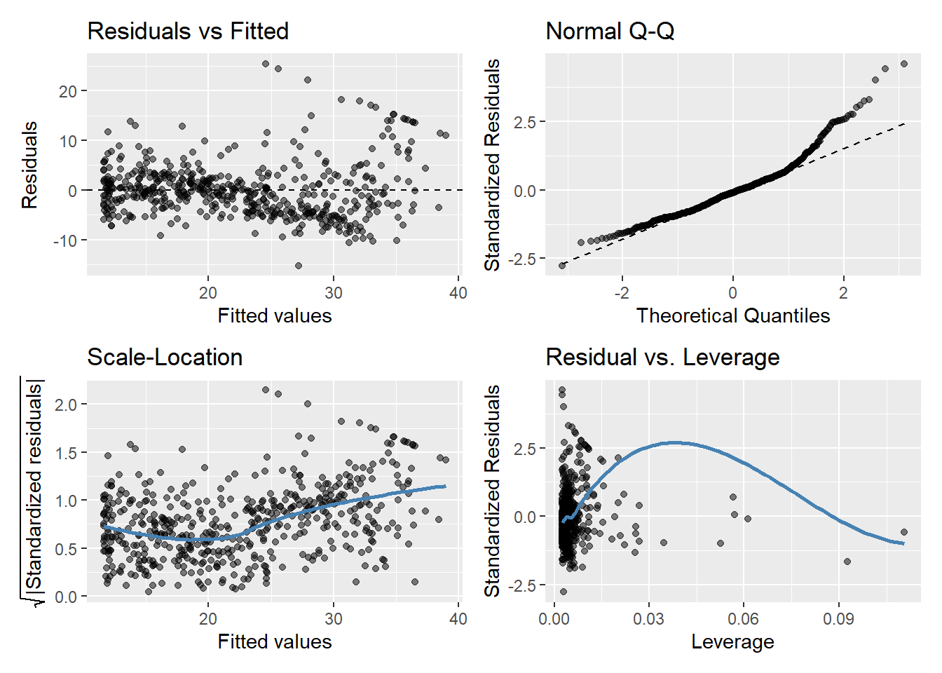
If we examine the diagnostic plots for the model with lstat^2, we will see little discernable pattern in the residuals:
par(mfrow =c(2,2))plot(lm.fit_quadratic)
Model = lm(medv ~ lstat + I(lstat^2))
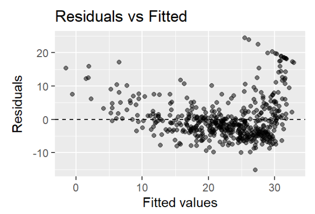
For reference, this is the Residuals vs Fitted Values plot of the original model, where lstat is not squared:
Model = lm(medv ~ lstat), for Residuals vs Fitted Values plot comparison.
We see that in the model with the transformed predictor, the distribution of residuals appears more evenly-spread with less of a discernable pattern, compared to the original. This is an improvement because it indicates there is less non-linearity in our new model!
More Polynomial Predictors
In order to create a cubic fit, we can include a predictor of the form I(X^3). However, this approach can start to get cumbersome for higher-order polynomials. A better approach involves using the poly() function to create the polynomial within lm(). For example, the following command produces a fifth-order polynomial fit:
This output suggests that including additional polynomial terms, up to fifth order, leads to an improvement in the model fit!
However, further investigation of the data reveals that no polynomial terms beyond fifth order have significant p-values in a regression fit.
By default, the poly() function orthogonalizes the predictors: this means that the features output by this function are not simply a sequence of powers of the argument. However, a linear model applied to the output of the poly() function will have the same fitted values as a linear model applied to the raw polynomials (although the coefficient estimates, standard errors, and p-values will differ). In order to obtain the raw polynomials from the poly() function, the argument raw = TRUE must be used.
Log Predictors
Of course, we are in no way restricted to using polynomial transformations of the predictors. Here we try a log transformation:
summary(lm(medv ~log(rm), data = Boston))
Call:
lm(formula = medv ~ log(rm), data = Boston)

Residuals:
    Min      1Q  Median      3Q     Max
-19.487  -2.875  -0.104   2.837  39.816

Coefficients:
            Estimate Std. Error t value Pr(>|t|)
(Intercept)  -76.488      5.028  -15.21   <2e-16 ***
log(rm)       54.055      2.739   19.73   <2e-16 ***
---
Signif. codes:  0 '***' 0.001 '**' 0.01 '*' 0.05 '.' 0.1 ' ' 1

Residual standard error: 6.915 on 504 degrees of freedom
Multiple R-squared:  0.4358,    Adjusted R-squared:  0.4347
F-statistic: 389.3 on 1 and 504 DF,  p-value: < 2.2e-16
Additional transformations for predictors include, but are not limited to:
The reciprocal: 1/X
Square root: \sqrt{X}
Qualitative Predictors
So far, we’ve looked at numerical data in our analysis, but what about categorical data? In the Carseats dataset, which is part of the ISLR2 library, we will attempt to predict Sales (child carseat sales) based on a number of predictors.
head(Carseats)
Sales
CompPrice
Income
Advertising
Population
Price
ShelveLoc
Age
Education
Urban
US
9.50
138
73
11
276
120
Bad
42
17
Yes
Yes
11.22
111
48
16
260
83
Good
65
10
Yes
Yes
10.06
113
35
10
269
80
Medium
59
12
Yes
Yes
7.40
117
100
4
466
97
Medium
55
14
Yes
Yes
4.15
141
64
3
340
128
Bad
38
13
Yes
No
10.81
124
113
13
501
72
Bad
78
16
No
Yes
The Carseats dataset includes qualitative predictors such as ShelveLoc, an indicator of the quality of the shelving location. The predictor ShelveLoc is a categorical factor that takes on three possible values: Good, Medium, and Bad.
Dummy variables and contrasts()
When given a qualitative variable such as ShelveLoc, R generates dummy variables automatically. Below we fit a multiple regression model that includes some interaction terms.
The contrasts() function returns the coding that R uses for the dummy variables.
Use the R command ?contrasts to learn about other contrasts, and how to set them.
attach(Carseats)contrasts(ShelveLoc)
       Good Medium
Bad       0      0
Good      1      0
Medium    0      1
As seen above:
R has created a ShelveLocGood dummy variable that takes on a value of 1 if the shelving location is good and 0 otherwise.
It has also created a ShelveLocMedium dummy variable that equals 1 if the shelving location is medium, and 0 otherwise.
A bad shelving location corresponds to a zero for each of the dummy variables.
The fact that the coefficient for ShelveLocGood in the regression output is positive indicates that a good shelving location is associated with high sales (relative to a bad location). ShelveLocMedium also has a positive coefficient, albeit smaller, indicating that a medium shelving location is also associated with higher sales than a bad shelving location, but lower than a good shelving location.
Model = lm(medv ~ lstat + I(lstat^2))Model = lm(medv ~ lstat), for Residuals vs Fitted Values plot comparison.